Ensemble Learning
from IPython.display import Image
Image('../../../python_for_probability_statistics_and_machine_learning.jpg')
from pprint import pprint
import textwrap
import sys, re
def displ(x):
   if x is None: return
   print ("\n".join(textwrap.wrap(repr(x).replace(' ',''),width=80)))

sys.displayhook=displ
With the exception of the random forest, we have so far considered machine learning models as stand-alone entities. Combinations of models that jointly produce a classification are known as ensembles. There are two main methodologies that create ensembles: bagging and boosting.
Bagging
Bagging refers to bootstrap aggregating, where bootstrap here is the same as we discussed in the section ch:stats:sec:boot. Basically, we resample the data with replacement and then train a classifier on the newly sampled data. Then, we combine the outputs of each of the individual classifiers using a majority-voting scheme (for discrete outputs) or a weighted average (for continuous outputs). This combination is particularly effective for models that are easily influenced by a single data element. The resampling process means that these elements cannot appear in every bootstrapped training set so that some of the models will not suffer these effects. This makes the so-computed combination of outputs less volatile. Thus, bagging helps reduce the collective variance of individual high-variance models.
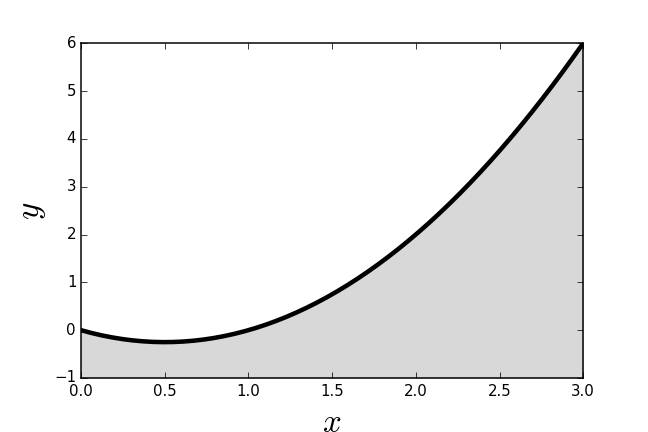
To get a sense of bagging, let's suppose we have a two-dimensional plane that is partitioned into two regions with the following boundary: $y=-x+x^2$. Pairs of $(x_i,y_i)$ points above this boundary are labeled one and points below are labeled zero. Figure shows the two regions with the nonlinear separating boundary as the black curved line.
Two regions in the plane are separated by a nonlinear boundary. The training data is sampled from this plane. The objective is to correctly classify the so- sampled data.

The problem is to take samples from each of these regions and classify them correctly using a perceptron. A perceptron is the simplest possible linear classifier that finds a line in the plane to separate two purported categories. Because the separating boundary is nonlinear, there is no way that the perceptron can completely solve this problem. The following code sets up the perceptron available in Scikit-learn.
from sklearn.linear_model import Perceptron
p=Perceptron()
p
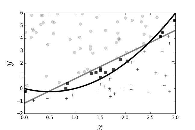
The training data and the resulting perceptron separating boundary are shown in Figure. The circles and crosses are the sampled training data and the gray separating line is the perceptron's separating boundary between the two categories. The black squares are those elements in the training data that the perceptron mis-classified. Because the perceptron can only produce linear separating boundaries, and the boundary in this case is non-linear, the perceptron makes mistakes near where the boundary curves. The next step is to see how bagging can improve upon this by using multiple perceptrons.
The perceptron finds the best linear boundary between the two classes.

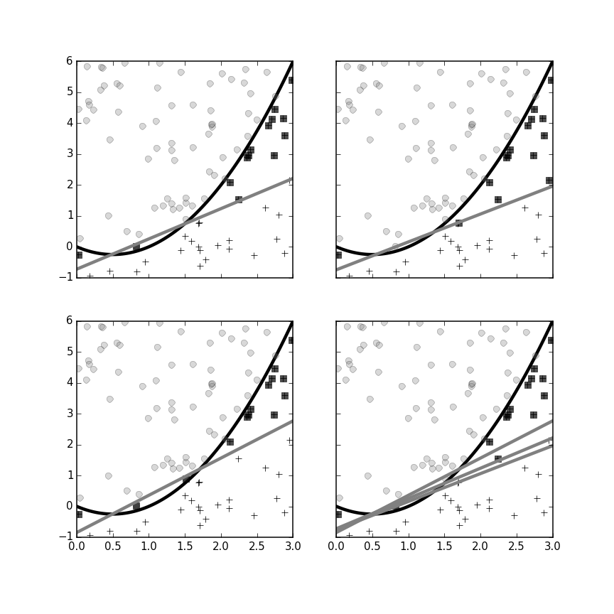
The following code sets up the bagging classifier in Scikit-learn. Here we select only three perceptrons. Figure shows each of the three individual classifiers and the final bagged classifer in the panel on the bottom right. As before, the black circles indicate misclassifications in the training data. Joint classifications are determined by majority voting.
from sklearn.ensemble import BaggingClassifier
bp = BaggingClassifier(Perceptron(),max_samples=0.50,n_estimators=3)
bp
Each panel with the single gray line is one of the perceptrons used for the ensemble bagging classifier on the lower right.

The BaggingClassifier can estimate its own out-of-sample error if passed the
oob_score=True flag upon construction. This keeps track of which samples were
used for training and which were not, and then estimates the out-of-sample
error using those samples that were unused in training. The max_samples
keyword argument specifies the number of items from the training set to use for
the base classifier. The smaller the max_samples used in the bagging
classifier, the better the out-of-sample error estimate, but at the cost of
worse in-sample performance. Of course, this depends on the overall number of
samples and the degrees-of-freedom in each individual classifier. The
VC-dimension surfaces again!
Boosting
As we discussed, bagging is particularly effective for individual high-variance classifiers because the final majority-vote tends to smooth out the individual classifiers and produce a more stable collaborative solution. On the other hand, boosting is particularly effective for high-bias classifiers that are slow to adjust to new data. On the one hand, boosting is similiar to bagging in that it uses a majority-voting (or averaging for numeric prediction) process at the end; and it also combines individual classifiers of the same type. On the other hand, boosting is serially iterative, whereas the individual classifiers in bagging can be trained in parallel. Boosting uses the misclassifications of prior iterations to influence the training of the next iterative classifier by weighting those misclassifications more heavily in subsequent steps. This means that, at every step, boosting focuses more and more on specific misclassifications up to that point, letting the prior classifications be carried by earlier iterations.
The primary implementation for boosting in Scikit-learn is the Adaptive
Boosting (AdaBoost) algorithm, which does classification
(AdaBoostClassifier) and regression (AdaBoostRegressor). The first step in
the basic AdaBoost algorithm is to initialize the weights over each of the
training set indicies, $D_0(i)=1/n$ where there are $n$ elements in the
training set. Note that this creates a discrete uniform distribution over the
indicies, not over the training data $\lbrace (x_i,y_i) \rbrace$ itself. In
other words, if there are repeated elements in the training data, then each
gets its own weight. The next step is to train the base classifer $h_k$ and
record the classification error at the $k^{th}$ iteration, $\epsilon_k$. Two
factors can next be calculated using $\epsilon_k$,
and the normalization factor,
$$ Z_k = 2 \sqrt{ \epsilon_k (1- \epsilon_k) } $$For the next step, the weights over the training data are updated as in the following,
$$ D_{k+1}(i) = \frac{1}{Z_k} D_k(i)\exp{(-\alpha_k y_i h_k(x_i))} $$The final classification result is assembled using the $\alpha_k$ factors, $g = \sgn(\sum_{k} \alpha_k h_k)$.
To re-do the problem above using boosting with perceptrons, we set up the AdaBoost classifier in the following,
from sklearn.ensemble import AdaBoostClassifier
clf=AdaBoostClassifier(Perceptron(),n_estimators=3,
                       algorithm='SAMME',
                       learning_rate=0.5)
clf
The learning_rate above controls how aggressively the weights are
updated. The resulting classification boundaries for the embedded perceptrons
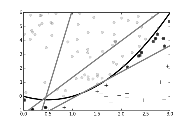
are shown in Figure. Compare this to the lower right
panel in Figure. The performance for both cases is about
the same. The IPython notebook corresponding to this section has more details
and the full listing of code used to produce all these figures.
The individual perceptron classifiers embedded in the AdaBoost classifier are shown along with the mis-classified points (in black). Compare this to the lower right panel of [Figure](#fig:ensemble_003).
