Regularization
from IPython.display import Image
Image('../../../python_for_probability_statistics_and_machine_learning.jpg')
We have referred to regularization in earlier sections, but we want to develop this important idea more fully. Regularization is the mechanism by which we navigate the bias/variance trade-off. To get started, let's consider a classic constrained least squares problem,
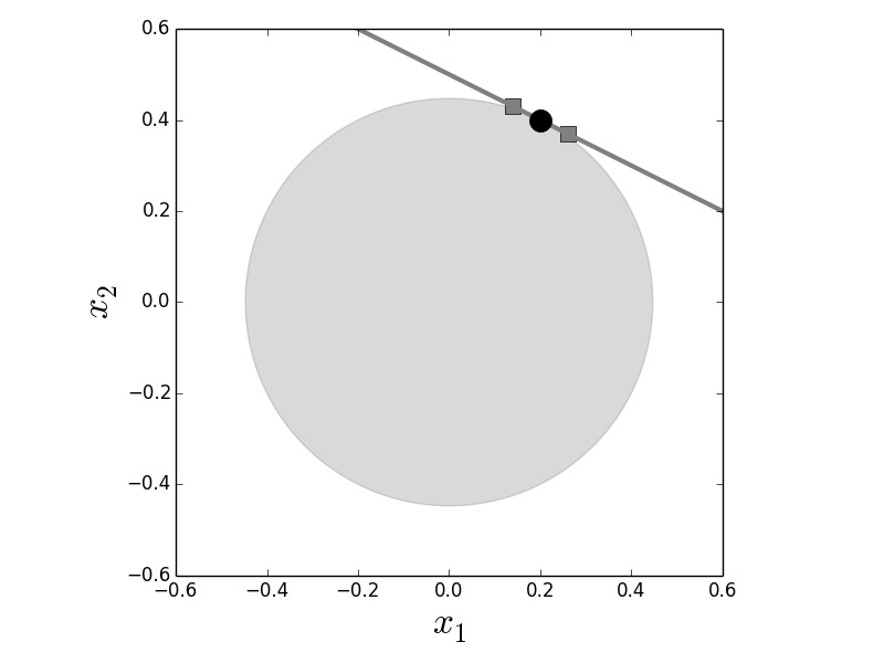
$$ \begin{aligned} & \underset{\mathbf{x}}{\text{minimize}} & & \Vert\mathbf{x}\Vert_2^2 \\ & \text{subject to:} & & x_0 + 2 x_1 = 1 \end{aligned} $$where $\Vert\mathbf{x}\Vert_2=\sqrt{x_0^2+x_1^2}$ is the $L_2$ norm. Without the constraint, it would be easy to minimize the objective function --- just take $\mathbf{x}=0$. Otherwise, suppose we somehow know that $\Vert\mathbf{x}\Vert_2<c$, then the locus of points defined by this inequality is the circle in Figure. The constraint is the line in the same figure. Because every value of $c$ defines a circle, the constraint is satisfied when the circle touches the line. The circle can touch the line at many different points, but we are only interested in the smallest such circle because this is a minimization problem. Intuitively, this means that we inflate a $L_2$ ball at the origin and stop when it just touches the contraint. The point of contact is our $L_2$ minimization solution.
The solution of the constrained $L_2$ minimization problem is at the point where the constraint (dark line) intersects the $L_2$ ball (gray circle) centered at the origin. The point of intersection is indicated by the dark circle. The two neighboring squares indicate points on the line that are close to the solution.

We can obtain the same result using the method of Lagrange multipliers. We can rewrite the entire $L_2$ minimization problem as one objective function using the Lagrange multiplier, $\lambda$,
$$ J(x_0,x_1,\lambda) = x_0^2+x_1^2 + \lambda (1-x_0-x_1) $$and solve this as an ordinary function using calculus. Let's do this using Sympy.
import sympy as S
S.var('x:2 l',real=True)
J=S.Matrix([x0,x1]).norm()**2 + l*(1-x0-2*x1)
sol=S.solve(map(J.diff,[x0,x1,l]))
print(sol)
Programming Tip.
Using the Matrix object is overkill for this problem but it
does demonstrate how Sympy's matrix machinery works. In this case,
we are using the norm method to compute the $L_2$ norm of the
given elements. Using S.var defines Sympy variables and injects
them into the global namespace. It is more Pythonic to do
something like x0 = S.symbols('x0',real=True) instead but the
other way is quicker, especially for variables with many
dimensions.
The solution defines the exact point where the line is tangent to the circle in Figure. The Lagrange multiplier has incorporated the constraint into the objective function.
%matplotlib inline

from __future__ import division
import numpy as np
from numpy import pi, linspace, sqrt
from matplotlib.patches import Circle
from matplotlib.pylab import subplots

x1 = linspace(-1,1,10)
dx=linspace(.7,1.3,3)
fline = lambda x:(1-x)/2.

fig,ax=subplots()
_=ax.plot(dx*1/5,fline(dx*1/5),'s',ms=10,color='gray')
_=ax.plot(x1,fline(x1),color='gray',lw=3)
_=ax.add_patch(Circle((0,0),1/sqrt(5),alpha=0.3,color='gray'))
_=ax.plot(1/5,2/5,'o',color='k',ms=15)
_=ax.set_xlabel('$x_1$',fontsize=24)
_=ax.set_ylabel('$x_2$',fontsize=24)
_=ax.axis((-0.6,0.6,-0.6,0.6))
ax.set_aspect(1)

fig.tight_layout()
There is something subtle and very important about the nature of the solution, however. Notice that there are other points very close to the solution on the circle, indicated by the squares in Figure. This closeness could be a good thing, in case it helps us actually find a solution in the first place, but it may be unhelpful in so far as it creates ambiguity. Let's hold that thought and try the same problem using the $L_1$ norm instead of the $L_2$ norm. Recall that
$$ \Vert \mathbf{x}\Vert_1 = \sum_{i=1}^d \vert x_i \vert $$where $d$ is the dimension of the vector $\mathbf{x}$. Thus, we can reformulate the same problem in the $L_1$ norm as in the following,
$$ \begin{aligned} & \underset{\mathbf{x}}{\text{minimize}} & & \Vert\mathbf{x}\Vert_1 \\ & \text{subject to:} & & x_1 + 2 x_2 = 1 \end{aligned} $$It turns out that this problem is somewhat harder to solve using Sympy, but we have convex optimization modules in Python that can help.
from cvxpy import Variable, Problem, Minimize, norm1, norm2
x=Variable(2,1,name='x')
constr=[np.matrix([[1,2]])*x==1]
obj=Minimize(norm1(x))
p= Problem(obj,constr)
p.solve()
print(x.value)
Programming Tip.
The cvxy module provides a unified and accessible interface to the powerful
cvxopt convex optimization package, as well as other open-source solver
packages.
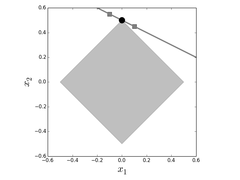
As shown in Figure, the constant-norm contour in the $L_1$ norm is shaped like a diamond instead of a circle. Furthermore, the solutions found in each case are different. Geometrically, this is because inflating the circular $L_2$ reaches out in all directions whereas the $L_1$ ball creeps out along the principal axes. This effect is much more pronounced in higher dimensional spaces where $L_1$-balls get more spikey 1. Like the $L_2$ case, there are also neighboring points on the constraint line, but notice that these are not close to the boundary of the corresponding $L_1$ ball, as they were in the $L_2$ case. This means that these would be harder to confuse with the optimal solution because they correspond to a substantially different $L_1$ ball.
when we covered the curse of dimensionality in the statistics chapter.
To double-check our earlier $L_2$ result, we can also use the
cvxpy module to find the $L_2$ solution as in the following
code,
We discussed the geometry of high dimensional space↩
constr=[np.matrix([[1,2]])*x==1]
obj=Minimize(norm2(x)) #L2 norm
p= Problem(obj,constr)
p.solve()
print(x.value)
The only change to the code is the $L_2$ norm and we get the same solution as before.
Let's see what happens in higher dimensions for both $L_2$ and $L_1$ as we move from two dimensions to four dimensions.
x=Variable(4,1,name='x')
constr=[np.matrix([[1,2,3,4]])*x==1]
obj=Minimize(norm1(x))
p= Problem(obj,constr)
p.solve()
print(x.value)
And also in the $L_2$ case with the following code,
constr=[np.matrix([[1,2,3,4]])*x==1]
obj=Minimize(norm2(x))
p= Problem(obj,constr)
p.solve()
print(x.value)
Note that the $L_1$ solution has selected out only one dimension for the solution, as the other components are effectively zero. This is not so with the $L_2$ solution, which has meaningful elements in multiple coordinates. This is because the $L_1$ problem has many pointy corners in the four dimensional space that poke at the hyperplane that is defined by the constraint. This essentially means the subsets (namely, the points at the corners) are found as solutions because these touch the hyperplane. This effect becomes more pronounced in higher dimensions, which is the main benefit of using the $L_1$ norm as we will see in the next section.
from matplotlib.patches import Rectangle, RegularPolygon

r=RegularPolygon((0,0),4,1/2,pi/2,alpha=0.5,color='gray')
fig,ax=subplots()
dx = np.array([-0.1,0.1])
_=ax.plot(dx,fline(dx),'s',ms=10,color='gray')
_=ax.plot(x1,fline(x1),color='gray',lw=3)
_=ax.plot(0,1/2,'o',color='k',ms=15)
_=ax.add_patch(r)
_=ax.set_xlabel('$x_1$',fontsize=24)
_=ax.set_ylabel('$x_2$',fontsize=24)
_=ax.axis((-0.6,0.6,-0.6,0.6))
_=ax.set_aspect(1)
fig.tight_layout()
The diamond is the $L_1$ ball in two dimensions and the line is the constraint. The point of intersection is the solution to the optimization problem. Note that for $L_1$ optimization, the two nearby points on the constraint (squares) do not touch the $L_1$ ball. Compare this with [Figure](#fig:regularization_001).

Ridge Regression
Now that we have a sense of the geometry of the situation, let's revisit our classic linear regression probem. To recap, we want to solve the following problem,
$$ \min_{\boldsymbol{\beta}\in \mathbb{R}^p} \Vert y - \mathbf{X}\boldsymbol{\beta}\Vert $$where $\mathbf{X}=\left[ \mathbf{x}_1,\mathbf{x}_2,\ldots,\mathbf{x}_p \right]$ and $\mathbf{x}_i\in \mathbb{R}^n$. Furthermore, we assume that the $p$ column vectors are linearly independent (i.e., $\texttt{rank}(\mathbf{X})=p$). Linear regression produces the $\boldsymbol{\beta}$ that minimizes the mean squared error above. In the case where $p=n$, there is a unique solution to this problem. However, when $p<n$, then there are infinitely many solutions.
To make this concrete, let's work this out using Sympy. First, let's define an example $\mathbf{X}$ and $\mathbf{y}$ matrix,
import sympy as S
from sympy import Matrix
X = Matrix([[1,2,3],
            [3,4,5]])
y = Matrix([[1,2]]).T
Now, we can define our coefficient vector $\boldsymbol{\beta}$ using the following code,
b0,b1,b2=S.symbols('b:3',real=True)
beta = Matrix([[b0,b1,b2]]).T # transpose
Next, we define the objective function we are trying to minimize
obj=(X*beta -y).norm(ord=2)**2
Programming Tip.
The Sympy Matrix class has useful methods like the norm function
used above to define the objective function. The ord=2 means we want
to use the $L_2$ norm. The expression in parenthesis evaluates to a
Matrix object.
Note that it is helpful to define real variables using the keyword argument whenever applicable because it relieves Sympy's internal machinery of dealing with complex numbers. Finally, we can use calculus to solve this by setting the derivatives of the objective function to zero.
sol=S.solve([obj.diff(i) for i in beta])
beta.subs(sol)
Notice that the solution does not uniquely specify all the components
of the beta variable. This is a consequence of the $p<n$ nature of this
problem where $p=2$ and $n=3$. While the the existence of this ambiguity does
not alter the solution,
obj.subs(sol)
But it does change the length of the solution vector
beta,
beta.subs(sol).norm(2)
If we want to minimize this length we can easily use the same calculus as before,
S.solve((beta.subs(sol).norm()**2).diff())
This provides the solution of minimum length in the $L_2$ sense,
betaL2=beta.subs(sol).subs(b2,S.Rational(1,6))
betaL2
But what is so special about solutions of minimum length? For machine learning, driving the objective function to zero is symptomatic of overfitting the data. Usually, at the zero bound, the machine learning method has essentially memorized the training data, which is bad for generalization. Thus, we can effectively stall this problem by defining a region for the solution that is away from the zero-bound.
$$ \begin{aligned} & \underset{\boldsymbol{\beta}}{\text{minimize}} & & \Vert y - \mathbf{X}\boldsymbol{\beta}\Vert_2^2 \\ & \text{subject to:} & & \Vert\boldsymbol{\beta}\Vert_2 < c \end{aligned} $$where $c$ is the tuning parameter. Using the same process as before, we can re-write this as the following,
$$ \min_{\boldsymbol{\beta}\in\mathbb{R}^p}\Vert y-\mathbf{X}\boldsymbol{\beta}\Vert_2^2 +\alpha\Vert\boldsymbol{\beta}\Vert_2^2 $$where $\alpha$ is the tuning parameter. These are the penalized or
Lagrange forms of these problems derived from the constrained versions. The
objective function is penalized by the $\Vert\boldsymbol{\beta}\Vert_2$ term.
For $L_2$ penalization, this is called ridge regression. This is
implemented in Scikit-learn as Ridge. The following code sets this up for
our example,
from sklearn.linear_model import Ridge
clf = Ridge(alpha=100.0,fit_intercept=False)
clf.fit(np.array(X).astype(float),np.array(y).astype(float))
Note that the alpha scales of the penalty for the
$\Vert\boldsymbol{\beta}\Vert_2$. We set the fit_intercept=False argument to
omit the extra offset term from our example. The corresponding solution is the
following,
print(clf.coef_)
To double-check the solution, we can use some optimization tools from Scipy and our previous Sympy analysis, as in the following,
from scipy.optimize import minimize
f   = S.lambdify((b0,b1,b2),obj+beta.norm()**2*100.)
g   = lambda x:f(x[0],x[1],x[2])
out = minimize(g,[.1,.2,.3]) # initial guess
out.x
Programming Tip.
We had to define the additional g function from the lambda function we
created from the Sympy expression in f because the minimize function
expects a single object vector as input instead of a three separate arguments.
which produces the same answer as the Ridge object. To
better understand the meaning of this result, we can re-compute the
mean squared error solution to this problem in one step using matrix
algebra instead of calculus,
betaLS=X.T*(X*X.T).inv()*y
betaLS
Notice that this solves the posited problem exactly,
X*betaLS-y
This means that the first term in the objective function goes to zero,
$$ \Vert y-\mathbf{X}\boldsymbol{\beta}_{LS}\Vert=0 $$But, let's examine the $L_2$ length of this solution versus the ridge regression solution,
print(betaLS.norm().evalf(), np.linalg.norm(clf.coef_))
Thus, the ridge regression solution is shorter in the $L_2$ sense, but the first term in the objective function is not zero for ridge regression,
print((y-X*clf.coef_.T).norm()**2)
Ridge regression solution trades fitting error ($\Vert y-\mathbf{X} \boldsymbol{\beta}\Vert_2$) for solution length ($\Vert\boldsymbol{\beta}\Vert_2$).
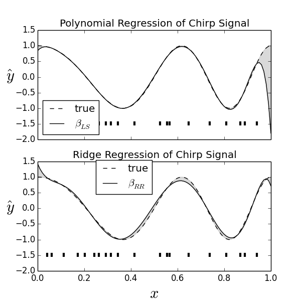
Let's see this in action with a familiar example from ch:stats:sec:nnreg. Consider Figure. For this example, we created our usual chirp signal and attempted to fit it with a high-dimensional polynomial, as we did in the section ch:ml:sec:cv. The lower panel is the same except with ridge regression. The shaded gray area is the space between the true signal and the approximant in both cases. The horizontal hash marks indicate the subset of $x_i$ values that each regressor was trained on. Thus, the training set represents a non-uniform sample of the underlying chirp waveform. The top panel shows the usual polynomial regression. Note that the regressor fits the given points extremely well, but fails at the endpoint. The ridge regressor misses many of the points in the middle, as indicated by the gray area, but does not overshoot at the ends as much as the plain polynomial regression. This is the basic trade-off for ridge regression. The Jupyter/IPython notebook has the code for this graph, but the main steps are shown in the following,
# create chirp signal
xi = np.linspace(0,1,100)[:,None]
# sample chirp randomly
xin= np.sort(np.random.choice(xi.flatten(),20,replace=False))[:,None]
# create sampled waveform
y = cos(2*pi*(xin+xin**2))
# create full waveform for reference
yi = cos(2*pi*(xi+xi**2))

# create polynomial features
qfit = PolynomialFeatures(degree=8) # quadratic
Xq = qfit.fit_transform(xin)
# reformat input as polynomial
Xiq = qfit.fit_transform(xi)

lr=LinearRegression() # create linear model
lr.fit(Xq,y) # fit linear model

# create ridge regression model and fit
clf = Ridge(alpha=1e-9,fit_intercept=False)
clf.fit(Xq,y)
from sklearn.preprocessing import PolynomialFeatures
from sklearn.linear_model import LinearRegression
import numpy as np
from numpy import cos, pi

np.random.seed(1234567)
xi = np.linspace(0,1,100)[:,None]
xin = np.linspace(0,1,20)[:,None]
xin= np.sort(np.random.choice(xi.flatten(),20,replace=False))[:,None]
f0 = 1 # init frequency
BW = 2
y = cos(2*pi*(f0*xin+(BW/2.0)*xin**2))
yi = cos(2*pi*(f0*xi+(BW/2.0)*xi**2))

qfit = PolynomialFeatures(degree=8) # quadratic
Xq = qfit.fit_transform(xin)
Xiq = qfit.fit_transform(xi)

lr=LinearRegression() # create linear model
_=lr.fit(Xq,y)

fig,axs=subplots(2,1,sharex=True,sharey=True)
fig.set_size_inches((6,6))
ax=axs[0]
_=ax.plot(xi,yi,label='true',ls='--',color='k')
_=ax.plot(xi,lr.predict(Xiq),label=r'$\beta_{LS}$',color='k')
_=ax.legend(loc=0)
_=ax.set_ylabel(r'$\hat{y}$  ',fontsize=22,rotation='horizontal')
_=ax.fill_between(xi.flatten(),yi.flatten(),lr.predict(Xiq).flatten(),color='gray',alpha=.3)
_=ax.set_title('Polynomial Regression of Chirp Signal')
_=ax.plot(xin, -1.5+np.array([0.01]*len(xin)), '|', color='k',mew=3)

clf = Ridge(alpha=1e-9,fit_intercept=False)
_=clf.fit(Xq,y)
ax=axs[1]
_=ax.plot(xi,yi,label=r'true',ls='--',color='k')
_=ax.plot(xi,clf.predict(Xiq),label=r'$\beta_{RR}$',color='k')
_=ax.legend(loc=(0.25,0.70))
_=ax.fill_between(xi.flatten(),yi.flatten(),clf.predict(Xiq).flatten(),color='gray',alpha=.3)
# add rug plot
_=ax.plot(xin, -1.5+np.array([0.01]*len(xin)), '|', color='k',mew=3)
_=ax.set_xlabel('$x$',fontsize=22)
_=ax.set_ylabel(r'$\hat{y}$  ',fontsize=22,rotation='horizontal')
_=ax.set_title('Ridge Regression of Chirp Signal')
The top figure shows polynomial regression and the lower panel shows polynomial ridge regression. The ridge regression does not match as well throughout most of the domain, but it does not flare as violently at the ends. This is because the ridge constraint holds the coefficient vector down at the expense of poorer performance along the middle of the domain.

Lasso
Lasso regression follows the same basic pattern as ridge regression, except with the $L_1$ norm in the objective function.
$$ \min_{\boldsymbol{\beta}\in\mathbb{R}^p}\Vert y-\mathbf{X}\boldsymbol{\beta}\Vert^2 +\alpha\Vert\boldsymbol{\beta}\Vert_1 $$The interface in Scikit-learn is likewise the same. The following is the same problem as before using lasso instead of ridge regression,
X = np.matrix([[1,2,3],
               [3,4,5]])
y = np.matrix([[1,2]]).T
from sklearn.linear_model import Lasso
lr = Lasso(alpha=1.0,fit_intercept=False)
_=lr.fit(X,y)
print(lr.coef_)
As before, we can use the optimization tools in Scipy to solve this also,
from scipy.optimize import fmin
obj = 1/4.*(X*beta-y).norm(2)**2 + beta.norm(1)*l
f = S.lambdify((b0,b1,b2),obj.subs(l,1.0))
g = lambda x:f(x[0],x[1],x[2])
fmin(g,[0.1,0.2,0.3])
Programming Tip.
The fmin function from Scipy's optimization module uses an
algorithm that does not depend upon derivatives. This is useful
because, unlike the $L_2$ norm, the $L_1$ norm has sharp corners
that make it harder to estimate derivatives.
This result matches the previous one from the
Scikit-learn Lasso object. Solving it using Scipy is motivating
and provides a good sanity check, but specialized algorithms are
required in practice. The following code block re-runs the lasso
with varying $\alpha$ and plots the coefficients in
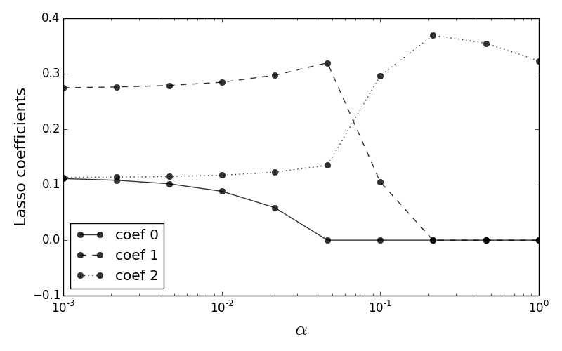
Figure. Notice that as $\alpha$ increases, all
but one of the coefficients is driven to zero. Increasing $\alpha$
makes the trade-off between fitting the data in the $L_2$ sense
and wanting to reduce the number of nonzero coefficients
(equivalently, the number of features used) in the model. For a
given problem, it may be more practical to focus on reducing the
number of features in the model (i.e., large $\alpha$) than the
quality of the data fit in the training data. The lasso provides a
clean way to navigate this trade-off.
The following code loops over a set of $\alpha$ values and collects the corresponding lasso coefficients to be plotted in Figure
o=[]
alphas= np.logspace(-3,0,10)
for a in alphas:
    clf = Lasso(alpha=a,fit_intercept=False)
    _=clf.fit(X,y)
    o.append(clf.coef_)
fig,ax=subplots()
fig.set_size_inches((8,5))
k=np.vstack(o)
ls = ['-','--',':','-.']
for i in range(k.shape[1]):
    _=ax.semilogx(alphas,k[:,i],'o-',
                label='coef %d'%(i),
                color='k',ls=ls[i],
                alpha=.8,)

_=ax.axis(ymin=-1e-1)
_=ax.legend(loc=0)
_=ax.set_xlabel(r'$\alpha$',fontsize=20)
_=ax.set_ylabel(r'Lasso coefficients',fontsize=16)
fig.tight_layout()
As $\alpha$ increases, more of the model coefficients are driven to zero for lasso regression.
