from IPython.display import Image
Image('../../../python_for_probability_statistics_and_machine_learning.jpg')
Information Entropy
We are in a position to discuss information entropy. This will give us a powerful perspective on how information passes between experiments, and will prove important in certain machine learning algorithms.
There used to be a TV game show where the host would hide a prize behind one of three doors and the contestant would have to pick one of the doors. However, before opening the door of the contestant's choice, the host would open one of the other doors and ask the contestant if she wanted to change her selection. This is the classic Monty Hall problem. The question is should the contestant stay with her original choice or switch after seeing what the host has revealed? From the information theory perspective, does the information environment change when the host reveals what is behind one of the doors? The important detail here is that the host never opens the door with the prize behind it, regardless of the contestant's choice. That is, the host knows where the prize is, but he does not reveal that information directly to the contestant. This is the fundamental problem information theory addresses --- how to aggregate and reason about partial information. We need a concept of information that can accommodate this kind of question.
Information Theory Concepts
The Shannon information content of an outcome $x$ is defined as,
where $P(x)$ is the probability of $x$. The entropy of the ensemble $X$ is defined to be the Shannon information content of
It is no accident that the entropy has this functional form as the expectation of $h(x)$. It leads to a deep and powerful theory of information.
To get some intuition about what information entropy means, consider a sequence of three-bit numbers where each individual bit is equally likely. Thus, the individual information content of a single bit is $h(x) = \log_2 (2) = 1$. The units of entropy are bits so this says that information content of a single bit is one bit. Because the three-bit number has elements that are mutually independent and equally likely, the information entropy of the three-bit number is $h(X) = 2^3 \times \log_2(2^3)/8=3 $. Thus, the basic idea of information content at least makes sense at this level.
A better way to interpret this question is as how much information would I have to provide in order to uniquely encode an arbitrary three-bit number? In this case, you would have to answer three questions: Is the first bit zero or one? Is the second bit zero or one? Is the third bit zero or one? Answering these questions uniquely specifies the unknown three-bit number. Because the bits are mutually independent, knowing the state of any of the bits does not inform the remainder.
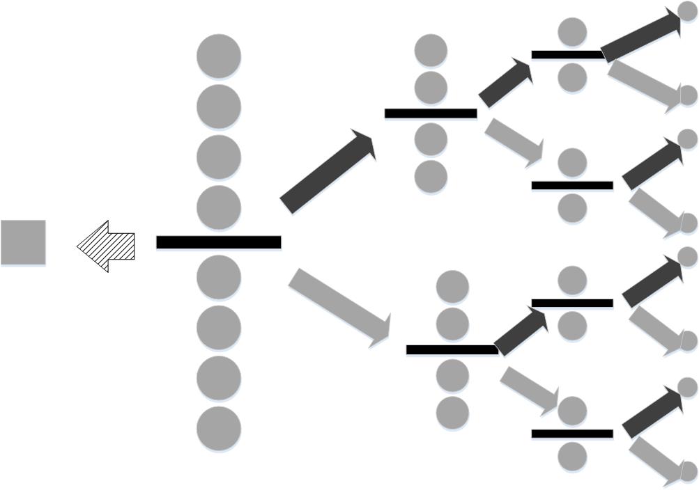
Next, let's consider a situation that lacks this mutual independence. Suppose in a group of nine otherwise identical balls there is a heavier one. Furthermore, we also have a measuring scale that indicates whether one side is heavier, lighter, or equal to the other. How could we identify the heavier ball? At the outset, the information content, which measures the uncertainty of the situation is $\log_2(9)$ because one of the nine balls is heavier. Figure shows one strategy. We could arbitrarily select out one of the balls (shown by the square), leaving the remaining eight to be balanced. The thick, black horizontal line indicates the scale. The items below and above this line indicate the counterbalanced sides of the scale.
One heavy ball is hidden among eight identical balls. By weighing groups sequentially, we can determine the heavy ball.

If we get lucky, the scale will report that the group of four walls on either side of the balance are equal in weight. This means that the ball that was omitted is the heavier one. This is indicated by the hashed left-pointing arrow. In this case, all the uncertainty has evaporated, and the informational value of that one weighing is equal to $\log_2(9)$. In other words, the scale has reduced the uncertainty to zero (i.e., found the heavy ball). On the other hand, the scale could report that the upper group of four balls is heavier (black, upward-pointing arrow) or lighter (gray, downward-pointing arrow). In this case, we cannot isolate the heavier ball until we perform all of the indicated weighings, moving from left-to-right. Specifically, the four balls on the heavier side have to be split by a subsequent weighing into two balls and then to one ball before the heavy ball can be identified. Thus, this process takes three weighings. The first one has information content $\log_2(9/8)$, the next has $\log_2(4)$, and the final one has $\log_2(2)$. Adding all these up sums to $\log_2(9)$. Thus, whether or not the heavier ball is isolated in the first weighing, the strategy consumes $\log_2(9)$ bits, as it must, to find the heavy ball.
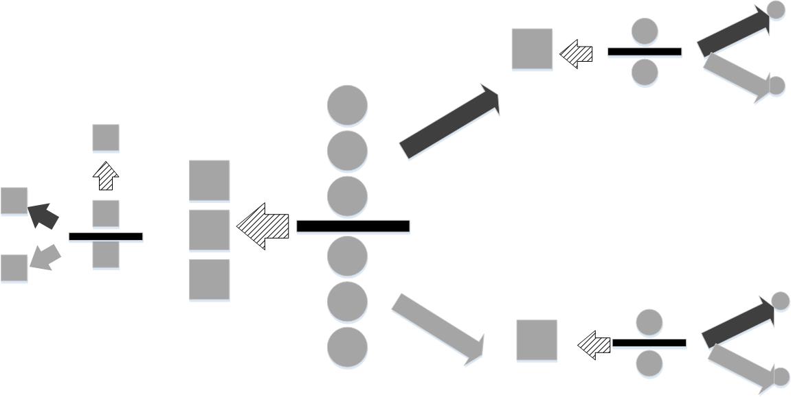
For this strategy, the balls are broken up into three groups of equal size and subsequently weighed.

However, this is not the only strategy. Figure shows another. In this approach, the nine balls are split up into three groups of three balls apiece. Two groups are weighed. If they are of equal weight, then this means the heavier ball is in the group that was left out (dashed arrow). Then, this group is split into two groups, with one element left out. If the two balls on the scale weigh the same, then it means the excluded one is the heavy one. Otherwise, it is one of the balls on the scale. The same process follows if one of the initially weighed groups is heavier (black upward-facing arrow) or lighter (gray lower-facing arrow). As before the information content of the situation is $\log_2(9)$. The first weighing reduces the uncertainty of the situation by $\log_2(3)$ and the subsequent weighing reduces it by another $\log_2(3)$. As before, these sum to $\log_2(9)$, but here we only need two weighings whereas the first strategy in Figure takes an average of $1/9 + 3*8/9 \approx 2.78$ weighings, which is more than two.
Why does the second strategy use fewer weighings? To reduce weighings, we need each weighing to adjudicate equally probable situations as many times as possible. Choosing one of the nine balls at the outset (i.e, first strategy in Figure) does not do this because the probability of selecting the correct ball is $1/9$. This does not create a equiprobable situation in the process. The second strategy leaves an equally probable situation at every stage (see Figure), so it extracts the most information out of each weighing as possible. Thus, the information content tells us how many bits of information have to be resolved using any strategy (i.e., $\log_2(9)$ in this example). It also illuminates how to efficiently remove uncertainty; namely, by adjudicating equiprobable situations as many times as possible.
Properties of Information Entropy
Now that we have the flavor of the concepts, consider the following properties of the information entropy,
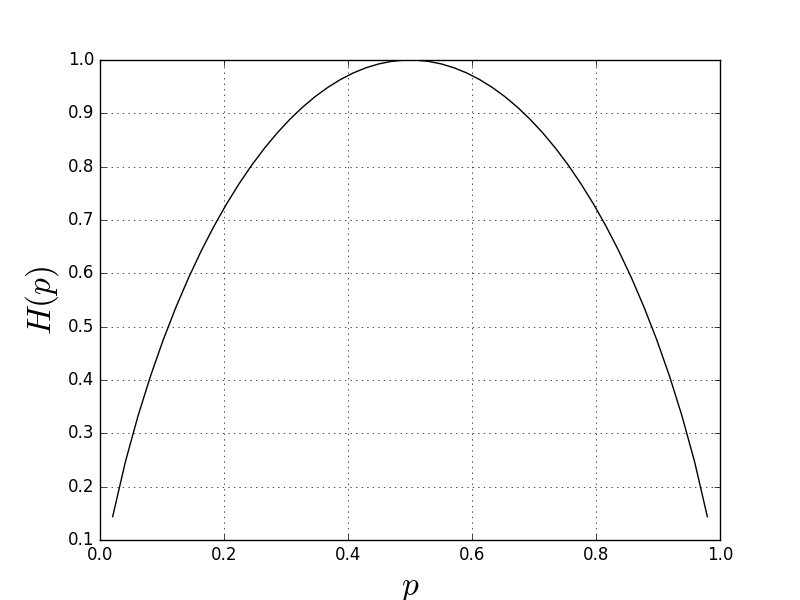
with equality if and only if $P(x)=1$ for exactly one $x$. Intuitively, this means that when just one of the items in the ensemble is known absolutely (i.e., with $P(x)=1$), the uncertainty collapses to zero. Also note that entropy is maximized when $P$ is uniformly distributed across the elements of the ensemble. This is illustrated in Figure for the case of two outcomes. In other words, information entropy is maximized when the two conflicting alternatives are equally probable. This is the mathematical reason why using the scale in the last example to adjudicate equally probable situations was so useful for abbreviating the weighing process.
%matplotlib inline

from matplotlib.pylab import subplots
import numpy as np
p = np.linspace(0,1,50)
fig,ax=subplots()
#fig.set_size_inches((14,7))
_=ax.plot(p,p*np.log2(1/p)+(1-p)*np.log2(1/(1-p)),'k-')
_=ax.set_xlabel('$p$',fontsize=24)
_=ax.set_ylabel('$H(p)$',fontsize=24)
_=ax.grid()
#fig.savefig('fig-probability/information_entropy_003.png')
The information entropy is maximized when $p=1/2$.

Most importantly, the concept of entropy extends jointly as follows,
If and only if $X$ and $Y$ are independent, entropy becomes additive,
Kullback-Leibler Divergence
Notions of information entropy lead to notions of distance between probability distributions that will become important for machine learning methods. The Kullback-Leibler divergence between two probability distributions $P$ and $Q$ that are defined over the same set is defined as,
Note that $D_{KL}(P,Q) \ge 0$ with equality if and only if $P=Q$. Sometimes the Kullback-Leibler divergence is called the Kullback-Leibler distance, but it is not formally a distance metric because it is asymmetrical in $P$ and $Q$. The Kullback-Leibler divergence defines a relative entropy as the loss of information if $P$ is modeled in terms of $Q$. There is an intuitive way to interpret the Kullback-Leibler divergence and understand its lack of symmetry. Suppose we have a set of messages to transmit, each with a corresponding probability $\lbrace (x_1,P(x_1)),(x_2,P(x_2)),\ldots,(x_n,P(x_n)) \rbrace$. Based on what we know about information entropy, it makes sense to encode the length of the message by $\log_2 \frac{1}{p(x)}$ bits. This parsimonious strategy means that more frequent messages are encoded with fewer bits. Thus, we can rewrite the entropy of the situation as before,
Now, suppose we want to transmit the same set of messages, but with a different set of probability weights, $\lbrace (x_1,Q(x_1)),(x_2,Q(x_2)),\ldots,(x_n,Q(x_n)) \rbrace$. In this situation, we can define the cross-entropy as
Note that only the purported length of the encoded message has changed, not the probability of that message. The difference between these two is the Kullback-Leibler divergence,
In this light, the Kullback-Leibler divergence is the average difference in the encoded lengths of the same set of messages under two different probability regimes. This should help explain the lack of symmetry of the Kullback-Leibler divergence --- left to themselves, $P$ and $Q$ would provide the optimal-length encodings separately, but there can be no necessary symmetry in how each regime would rate the informational value of each message ($Q(x_i)$ versus $P(x_i)$). Given that each encoding is optimal-length in its own regime means that it must therefore be at least sub-optimal in another, thus giving rise to the Kullback-Leibler divergence. In the case where the encoding length of all messages remains the same for the two regimes, then the Kullback-Leibler divergence is zero 1.
four of Mackay's text [mackay2003information]. Another good reference is chapter four of [hastie2013elements].
The best, easy-to-understand presentation of this material is chapter↩