In [2]:
from IPython.display import Image 
Image('../../../python_for_probability_statistics_and_machine_learning.jpg')
Out[2]:
In [3]:
from __future__ import division
%pylab  inline
Populating the interactive namespace from numpy and matplotlib

Monte Carlo Sampling Methods

So far, we have studied analytical ways to transform random variables and how to augment these methods using Python. In spite of all this, we frequently must resort to purely numerical methods to solve real-world problems. Hopefully, now that we have seen the deeper theory, these numerical methods feel more concrete. Suppose we want to generate samples of a given density, $f(x)$, given we already can generate samples from a uniform distribution, $\mathcal{U}[0,1]$. How do we know a random sample $v$ comes from the $f(x)$ distribution? One approach is to look at how a histogram of samples of $v$ approximates $f(x)$. Specifically,

$$ \begin{equation} \mathbb{P}( v \in N_{\Delta}(x) ) = f(x) \Delta x \end{equation} \label{eq:mc01} \tag{1} $$

The histogram approximates the target probability density.
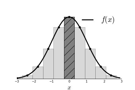
which says that the probability that a sample is in some $N_\Delta$ neighborhood of $x$ is approximately $f(x)\Delta x$. Figure shows the target probability density function $f(x)$ and a histogram that approximates it. The histogram is generated from samples $v$. The hatched rectangle in the center illustrates Equation ref{eq:mc01}. The area of this rectangle is approximately $f(x)\Delta x$ where $x=0$, in this case. The width of the rectangle is $N_{\Delta}(x)$ The quality of the approximation may be clear visually, but to know that $v$ samples are characterized by $f(x)$, we need the statement of Equation ref{eq:mc01}, which says that the proportion of samples $v$ that fill the hatched rectangle is approximately equal to $f(x)\Delta x$.

Now that we know how to evaluate samples $v$ that are characterized by the density $f(x)$, let's consider how to create these samples for both discrete and continuous random variables.

Inverse CDF Method for Discrete Variables

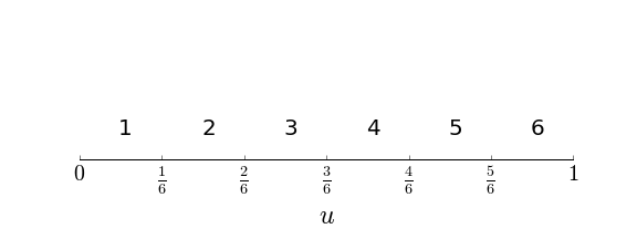
Suppose we want to generate samples from a fair six-sided die. Our workhouse uniform random variable is defined continuously over the unit interval and the fair six-sided die is discrete. We must first create a mapping between the continuous random variable $u$ and the discrete outcomes of the die. This mapping is shown in Figure where the unit interval is broken up into segments, each of length $1/6$. Each individual segment is assigned to one of the die outcomes. For example, if $u \in [1/6,2/6)$, then the outcome for the die is $2$. Because the die is fair, all segments on the unit interval are the same length. Thus, our new random variable $v$ is derived from $u$ by this assignment.

A uniform distribution random variable on the unit interval is assigned to the six outcomes of a fair die using these segements.
For example, for $v=2$, we have,

$$ \mathbb{P}(v=2) = \mathbb{P}(u\in [1/6,2/6)) = 1/6 $$

where, in the language of the Equation ref{eq:mc01}, $f(x)=1$ (uniform distribution), $\Delta x = 1/6$, and $N_\Delta (2)=[1/6,2/6)$. Naturally, this pattern holds for all the other die outcomes in $\left\{1,2,3,..,6\right\}$. Let's consider a quick simulation to make this concrete. The following code generates uniform random samples and stacks them in a Pandas dataframe.

In [4]:
import pandas as pd
import numpy as np
from pandas import DataFrame
u= np.random.rand(100)
df = DataFrame(data=u,columns=['u'])

The next block uses pd.cut to map the individual samples to the set $\left\{1,2,\ldots,6\right\}$ labeled v.

In [5]:
labels = [1,2,3,4,5,6]
df['v']=pd.cut(df.u,np.linspace(0,1,7),
               include_lowest=True,labels=labels)

This is what the dataframe contains. The v column contains the samples drawn from the fair die.

In [6]:
>>> df.head()
          
Out[6]:
u v
0 0.605368 4
1 0.525941 4
2 0.141985 1
3 0.729510 5
4 0.240505 2

The following is a count of the number of samples in each group. There should be roughly the same number of samples in each group because the die is fair.

In [7]:
>>> df.groupby('v').count()
    
Out[7]:
u
v
1 19
2 15
3 15
4 16
5 23
6 12

So far, so good. We now have a way to simulate a fair die from a uniformly distributed random variable.

To extend this to unfair die, we need only make some small adjustments to this code. For example, suppose that we want an unfair die so that $\mathbb{P}(1)=\mathbb{P}(2)=\mathbb{P}(3)=1/12$ and $\mathbb{P}(4)=\mathbb{P}(5)=\mathbb{P}(6)=1/4$. The only change we have to make is with pd.cut as follows,

In [8]:
df['v']=pd.cut(df.u,[0,1/12,2/12,3/12,2/4,3/4,1],
               include_lowest=True,labels=labels)
In [9]:
>>> df.groupby('v').count()/df.shape[0]
      
Out[9]:
u
v
1 0.05
2 0.14
3 0.07
4 0.23
5 0.32
6 0.19
u v 1 0.08 2 0.10 3 0.09 4 0.23 5 0.19 6 0.31

where now these are the individual probabilities of each digit. You can take more than 100 samples to get a clearer view of the individual probabilities but the mechanism for generating them is the same. The method is called the inverse CDF 1 method because the CDF (namely,$\texttt{[0,1/12,2/12,3/12,2/4,3/4,1]}$) in the last example has been inverted (using the pd.cut method) to generate the samples.
The inversion is easier to see for continuous variables, which we consider next.

Inverse CDF Method for Continuous Variables

The method above applies to continuous random variables, but now we have to use squeeze the intervals down to individual points. In the example above, our inverse function was a piecewise function that operated on uniform random samples. In this case, the piecewise function collapses to a continuous inverse function. We want to generate random samples for a CDF that is invertible. As before, the criterion for generating an appropriate sample $v$ is the following,


  1. Cumulative density function. Namely, $F(x)=\mathbb{P}(X < x)$.

$$ \mathbb{P}(F(x) < v < F(x+\Delta x)) = F(x+\Delta x) - F(x) = \int_x^{x+\Delta x} f(u) du \approx f(x) \Delta x $$

which is saying that the probability that the sample $v$ is contained in a $\Delta x$ interval is approximately equal to the density function, $f(x) \Delta x$, at that point. Once again, the trick is to use a uniform random sample $u$ and an invertible CDF $F(x)$ to construct these samples. Note that for a uniform random variable $u \sim \mathcal{U}[0,1]$, we have,

$$ \begin{align*} \mathbb{P}(x < F^{-1}(u) < x+\Delta x) & = \mathbb{P}(F(x) < u < F(x+\Delta x)) \\\ & = F(x+\Delta x) - F(x) \\\ & = \int_x^{x+\Delta x} f(p) dp \approx f(x) \Delta x \end{align*} $$

This means that $ v=F^{-1}(u) $ is distributed according to $f(x)$, which is what we want.

Let's try this to generate samples from the exponential distribution,

$$ f_{\alpha}(x) = \alpha e^{ -\alpha x } $$

which has the following CDF,

$$ F(x) = 1-e^{ -\alpha x } $$

and corresponding inverse,

$$ F^{-1}(u) = \frac{1}{\alpha}\ln \frac{1}{(1-u)} $$

Now, all we have to do is generate some uniformly distributed random samples and then feed them into $F^{-1}$.

In [10]:
from numpy import array, log
import scipy.stats
alpha = 1.   # distribution parameter
nsamp = 1000 # num of samples
# define uniform random variable
u=scipy.stats.uniform(0,1)
# define inverse function
Finv=lambda u: 1/alpha*log(1/(1-u))
# apply inverse function to samples
v = array(map(Finv,u.rvs(nsamp)))

Now, we have the samples from the exponential distribution, but how do we know the method is correct with samples distributed accordingly? Fortunately, scipy.stats already has a exponential distribution, so we can check our work against the reference using a probability plot (i.e., also known as a quantile-quantile plot). The following code sets up the probability plot from scipy.stats.

In [11]:
%matplotlib inline

from matplotlib.pylab import setp, subplots
fig,ax = subplots()
fig.set_size_inches((7,5))
_=scipy.stats.probplot(v,(1,),dist='expon',plot=ax)
line=ax.get_lines()[0]
_=setp(line,'color','k')
_=setp(line,'alpha',.1)
line=ax.get_lines()[1]
_=setp(line,'color','gray')
_=setp(line,'lw',3.0)
_=setp(ax.yaxis.get_label(),'fontsize',18)
_=setp(ax.xaxis.get_label(),'fontsize',18)
_=ax.set_title('Probability Plot',fontsize=18)
_=ax.grid()
fig.tight_layout()
#fig.savefig('fig-probability/Sampling_Monte_Carlo_005.png')
In [12]:
fig,ax=subplots()
scipy.stats.probplot(v,(1,),dist='expon',plot=ax)
Out[12]:
((array([ 1.00069315,  1.0016833 ,  1.00268512,  1.00368795,  1.00469178,
          1.00569662,  1.00670247,  1.00770934,  1.00871722,  1.00972611,
          1.01073603,  1.01174696,  1.01275892,  1.01377191,  1.01478592,
          1.01580096,  1.01681703,  1.01783414,  1.01885228,  1.01987145,
          1.02089167,  1.02191293,  1.02293524,  1.02395859,  1.02498299,
          1.02600844,  1.02703494,  1.02806249,  1.02909111,  1.03012078,
          1.03115151,  1.03218331,  1.03321617,  1.03425011,  1.03528511,
          1.03632118,  1.03735833,  1.03839655,  1.03943586,  1.04047624,
          1.04151771,  1.04256027,  1.04360391,  1.04464864,  1.04569447,
          1.04674139,  1.04778941,  1.04883852,  1.04988874,  1.05094006,
          1.05199249,  1.05304603,  1.05410068,  1.05515644,  1.05621332,
          1.05727132,  1.05833044,  1.05939068,  1.06045204,  1.06151454,
          1.06257816,  1.06364292,  1.06470881,  1.06577583,  1.066844  ,
          1.06791331,  1.06898377,  1.07005537,  1.07112812,  1.07220202,
          1.07327708,  1.0743533 ,  1.07543067,  1.07650921,  1.07758891,
          1.07866978,  1.07975181,  1.08083502,  1.08191941,  1.08300497,
          1.08409171,  1.08517963,  1.08626874,  1.08735904,  1.08845052,
          1.0895432 ,  1.09063708,  1.09173215,  1.09282842,  1.09392589,
          1.09502457,  1.09612446,  1.09722556,  1.09832788,  1.09943141,
          1.10053616,  1.10164213,  1.10274933,  1.10385775,  1.1049674 ,
          1.10607829,  1.10719041,  1.10830377,  1.10941837,  1.11053421,
          1.11165131,  1.11276965,  1.11388924,  1.11501008,  1.11613219,
          1.11725555,  1.11838018,  1.11950608,  1.12063324,  1.12176168,
          1.12289139,  1.12402238,  1.12515465,  1.1262882 ,  1.12742304,
          1.12855917,  1.12969659,  1.1308353 ,  1.13197532,  1.13311663,
          1.13425925,  1.13540318,  1.13654841,  1.13769496,  1.13884283,
          1.13999201,  1.14114252,  1.14229435,  1.14344751,  1.144602  ,
          1.14575782,  1.14691499,  1.14807349,  1.14923334,  1.15039453,
          1.15155708,  1.15272097,  1.15388623,  1.15505284,  1.15622082,
          1.15739016,  1.15856087,  1.15973295,  1.16090641,  1.16208124,
          1.16325746,  1.16443507,  1.16561406,  1.16679444,  1.16797622,
          1.1691594 ,  1.17034397,  1.17152996,  1.17271735,  1.17390615,
          1.17509637,  1.176288  ,  1.17748106,  1.17867554,  1.17987146,
          1.1810688 ,  1.18226758,  1.1834678 ,  1.18466945,  1.18587256,
          1.18707711,  1.18828312,  1.18949059,  1.19069951,  1.1919099 ,
          1.19312175,  1.19433507,  1.19554987,  1.19676614,  1.1979839 ,
          1.19920314,  1.20042387,  1.20164609,  1.20286981,  1.20409503,
          1.20532175,  1.20654997,  1.20777971,  1.20901096,  1.21024373,
          1.21147802,  1.21271383,  1.21395118,  1.21519005,  1.21643047,
          1.21767242,  1.21891592,  1.22016097,  1.22140757,  1.22265572,
          1.22390544,  1.22515672,  1.22640956,  1.22766398,  1.22891998,
          1.23017755,  1.23143671,  1.23269745,  1.23395978,  1.23522372,
          1.23648925,  1.23775638,  1.23902512,  1.24029548,  1.24156745,
          1.24284104,  1.24411625,  1.24539309,  1.24667156,  1.24795168,
          1.24923343,  1.25051682,  1.25180187,  1.25308857,  1.25437693,
          1.25566694,  1.25695863,  1.25825199,  1.25954702,  1.26084373,
          1.26214212,  1.2634422 ,  1.26474398,  1.26604745,  1.26735262,
          1.2686595 ,  1.26996809,  1.27127839,  1.27259041,  1.27390416,
          1.27521963,  1.27653684,  1.27785578,  1.27917647,  1.2804989 ,
          1.28182308,  1.28314902,  1.28447672,  1.28580619,  1.28713742,
          1.28847043,  1.28980522,  1.29114179,  1.29248015,  1.29382031,
          1.29516226,  1.29650602,  1.29785158,  1.29919896,  1.30054815,
          1.30189917,  1.30325202,  1.3046067 ,  1.30596321,  1.30732157,
          1.30868178,  1.31004384,  1.31140776,  1.31277354,  1.31414118,
          1.3155107 ,  1.3168821 ,  1.31825539,  1.31963056,  1.32100762,
          1.32238658,  1.32376745,  1.32515023,  1.32653492,  1.32792153,
          1.32931007,  1.33070054,  1.33209294,  1.33348729,  1.33488358,
          1.33628182,  1.33768203,  1.33908419,  1.34048833,  1.34189444,
          1.34330253,  1.3447126 ,  1.34612467,  1.34753873,  1.34895479,
          1.35037287,  1.35179295,  1.35321506,  1.35463919,  1.35606535,
          1.35749355,  1.35892379,  1.36035608,  1.36179043,  1.36322683,
          1.36466531,  1.36610585,  1.36754847,  1.36899318,  1.37043997,
          1.37188887,  1.37333986,  1.37479296,  1.37624818,  1.37770552,
          1.37916499,  1.38062658,  1.38209032,  1.38355621,  1.38502424,
          1.38649444,  1.38796679,  1.38944132,  1.39091803,  1.39239692,
          1.393878  ,  1.39536128,  1.39684676,  1.39833445,  1.39982436,
          1.40131649,  1.40281085,  1.40430745,  1.40580629,  1.40730738,
          1.40881073,  1.41031634,  1.41182422,  1.41333438,  1.41484682,
          1.41636155,  1.41787858,  1.41939792,  1.42091957,  1.42244353,
          1.42396983,  1.42549845,  1.42702942,  1.42856273,  1.4300984 ,
          1.43163643,  1.43317683,  1.43471961,  1.43626476,  1.43781232,
          1.43936226,  1.44091462,  1.44246939,  1.44402658,  1.4455862 ,
          1.44714825,  1.44871275,  1.4502797 ,  1.45184911,  1.45342099,
          1.45499534,  1.45657217,  1.4581515 ,  1.45973332,  1.46131765,
          1.46290449,  1.46449385,  1.46608575,  1.46768018,  1.46927716,
          1.47087669,  1.47247879,  1.47408345,  1.4756907 ,  1.47730053,
          1.47891296,  1.480528  ,  1.48214564,  1.48376591,  1.4853888 ,
          1.48701434,  1.48864252,  1.49027336,  1.49190686,  1.49354303,
          1.49518188,  1.49682343,  1.49846767,  1.50011462,  1.50176429,
          1.50341669,  1.50507181,  1.50672969,  1.50839031,  1.5100537 ,
          1.51171986,  1.5133888 ,  1.51506054,  1.51673507,  1.51841241,
          1.52009256,  1.52177555,  1.52346137,  1.52515004,  1.52684156,
          1.52853596,  1.53023322,  1.53193338,  1.53363642,  1.53534238,
          1.53705125,  1.53876304,  1.54047777,  1.54219545,  1.54391608,
          1.54563967,  1.54736624,  1.5490958 ,  1.55082836,  1.55256392,
          1.5543025 ,  1.5560441 ,  1.55778875,  1.55953645,  1.5612872 ,
          1.56304102,  1.56479793,  1.56655793,  1.56832103,  1.57008725,
          1.57185659,  1.57362906,  1.57540469,  1.57718347,  1.57896542,
          1.58075055,  1.58253888,  1.58433041,  1.58612515,  1.58792312,
          1.58972433,  1.59152879,  1.59333652,  1.59514751,  1.59696179,
          1.59877937,  1.60060026,  1.60242447,  1.60425202,  1.60608291,
          1.60791716,  1.60975478,  1.61159578,  1.61344018,  1.61528798,
          1.61713921,  1.61899387,  1.62085198,  1.62271354,  1.62457858,
          1.6264471 ,  1.62831912,  1.63019465,  1.63207371,  1.6339563 ,
          1.63584244,  1.63773215,  1.63962544,  1.64152231,  1.64342279,
          1.64532689,  1.64723463,  1.64914601,  1.65106105,  1.65297976,
          1.65490216,  1.65682827,  1.65875809,  1.66069165,  1.66262895,
          1.66457001,  1.66651484,  1.66846347,  1.6704159 ,  1.67237215,
          1.67433223,  1.67629616,  1.67826396,  1.68023564,  1.68221121,
          1.68419069,  1.6861741 ,  1.68816145,  1.69015276,  1.69214804,
          1.69414732,  1.69615059,  1.69815789,  1.70016922,  1.70218461,
          1.70420407,  1.70622761,  1.70825526,  1.71028703,  1.71232293,
          1.71436299,  1.71640722,  1.71845563,  1.72050825,  1.72256509,
          1.72462617,  1.72669151,  1.72876112,  1.73083503,  1.73291324,
          1.73499579,  1.73708267,  1.73917393,  1.74126956,  1.7433696 ,
          1.74547405,  1.74758295,  1.7496963 ,  1.75181412,  1.75393644,
          1.75606328,  1.75819465,  1.76033057,  1.76247106,  1.76461614,
          1.76676584,  1.76892016,  1.77107914,  1.77324279,  1.77541113,
          1.77758418,  1.77976196,  1.7819445 ,  1.78413181,  1.78632392,
          1.78852084,  1.7907226 ,  1.79292922,  1.79514071,  1.79735711,
          1.79957843,  1.8018047 ,  1.80403594,  1.80627216,  1.8085134 ,
          1.81075967,  1.813011  ,  1.8152674 ,  1.81752891,  1.81979555,
          1.82206734,  1.8243443 ,  1.82662645,  1.82891383,  1.83120645,
          1.83350433,  1.83580751,  1.83811601,  1.84042985,  1.84274905,
          1.84507365,  1.84740366,  1.84973911,  1.85208004,  1.85442645,
          1.85677838,  1.85913586,  1.86149891,  1.86386755,  1.86624182,
          1.86862174,  1.87100734,  1.87339864,  1.87579567,  1.87819846,
          1.88060705,  1.88302144,  1.88544168,  1.88786779,  1.8902998 ,
          1.89273774,  1.89518164,  1.89763153,  1.90008743,  1.90254938,
          1.9050174 ,  1.90749153,  1.9099718 ,  1.91245824,  1.91495087,
          1.91744973,  1.91995485,  1.92246626,  1.924984  ,  1.92750809,
          1.93003857,  1.93257547,  1.93511882,  1.93766865,  1.940225  ,
          1.94278791,  1.9453574 ,  1.94793351,  1.95051627,  1.95310572,
          1.95570189,  1.95830482,  1.96091455,  1.9635311 ,  1.96615452,
          1.96878484,  1.97142209,  1.97406632,  1.97671755,  1.97937584,
          1.98204121,  1.98471371,  1.98739336,  1.99008022,  1.99277431,
          1.99547568,  1.99818437,  2.00090042,  2.00362386,  2.00635474,
          2.0090931 ,  2.01183898,  2.01459242,  2.01735346,  2.02012214,
          2.02289851,  2.02568262,  2.02847449,  2.03127418,  2.03408173,
          2.03689719,  2.03972059,  2.04255199,  2.04539143,  2.04823896,
          2.05109461,  2.05395845,  2.05683051,  2.05971084,  2.06259949,
          2.06549651,  2.06840195,  2.07131585,  2.07423827,  2.07716925,
          2.08010885,  2.08305712,  2.08601411,  2.08897986,  2.09195444,
          2.09493789,  2.09793027,  2.10093163,  2.10394203,  2.10696151,
          2.10999014,  2.11302797,  2.11607506,  2.11913146,  2.12219723,
          2.12527243,  2.12835712,  2.13145134,  2.13455518,  2.13766868,
          2.1407919 ,  2.1439249 ,  2.14706776,  2.15022052,  2.15338325,
          2.15655602,  2.15973888,  2.16293191,  2.16613517,  2.16934872,
          2.17257263,  2.17580697,  2.17905181,  2.1823072 ,  2.18557323,
          2.18884996,  2.19213746,  2.19543581,  2.19874507,  2.20206532,
          2.20539663,  2.20873908,  2.21209273,  2.21545767,  2.21883397,
          2.22222171,  2.22562096,  2.22903181,  2.23245433,  2.23588861,
          2.23933472,  2.24279274,  2.24626277,  2.24974488,  2.25323916,
          2.25674569,  2.26026456,  2.26379585,  2.26733966,  2.27089608,
          2.27446518,  2.27804707,  2.28164184,  2.28524957,  2.28887037,
          2.29250433,  2.29615154,  2.2998121 ,  2.30348611,  2.30717367,
          2.31087487,  2.31458983,  2.31831864,  2.3220614 ,  2.32581823,
          2.32958922,  2.33337448,  2.33717413,  2.34098828,  2.34481702,
          2.34866048,  2.35251877,  2.35639201,  2.3602803 ,  2.36418377,
          2.36810254,  2.37203673,  2.37598645,  2.37995184,  2.38393301,
          2.3879301 ,  2.39194323,  2.39597253,  2.40001813,  2.40408016,
          2.40815876,  2.41225406,  2.41636621,  2.42049533,  2.42464157,
          2.42880508,  2.432986  ,  2.43718446,  2.44140063,  2.44563465,
          2.44988668,  2.45415686,  2.45844535,  2.46275231,  2.46707791,
          2.47142229,  2.47578563,  2.4801681 ,  2.48456985,  2.48899107,
          2.49343192,  2.49789258,  2.50237322,  2.50687403,  2.5113952 ,
          2.51593689,  2.52049931,  2.52508263,  2.52968706,  2.53431279,
          2.53896002,  2.54362894,  2.54831977,  2.5530327 ,  2.55776795,
          2.56252573,  2.56730625,  2.57210974,  2.57693641,  2.58178649,
          2.58666021,  2.5915578 ,  2.5964795 ,  2.60142553,  2.60639616,
          2.61139161,  2.61641214,  2.621458  ,  2.62652946,  2.63162676,
          2.63675019,  2.64189999,  2.64707646,  2.65227985,  2.65751047,
          2.66276859,  2.6680545 ,  2.67336851,  2.6787109 ,  2.68408199,
          2.68948208,  2.69491149,  2.70037054,  2.70585955,  2.71137887,
          2.71692881,  2.72250972,  2.72812196,  2.73376588,  2.73944182,
          2.74515017,  2.75089129,  2.75666556,  2.76247337,  2.76831511,
          2.77419117,  2.78010196,  2.7860479 ,  2.79202941,  2.79804691,
          2.80410083,  2.81019164,  2.81631976,  2.82248568,  2.82868984,
          2.83493274,  2.84121486,  2.84753669,  2.85389875,  2.86030154,
          2.86674558,  2.87323143,  2.87975961,  2.88633069,  2.89294524,
          2.89960383,  2.90630705,  2.91305551,  2.91984983,  2.92669062,
          2.93357853,  2.94051421,  2.94749833,  2.95453157,  2.96161463,
          2.96874822,  2.97593306,  2.9831699 ,  2.99045949,  2.99780261,
          3.00520006,  3.01265263,  3.02016116,  3.02772649,  3.0353495 ,
          3.04303106,  3.05077208,  3.0585735 ,  3.06643626,  3.07436133,
          3.08234971,  3.09040241,  3.0985205 ,  3.10670502,  3.11495708,
          3.12327781,  3.13166835,  3.14012989,  3.14866364,  3.15727084,
          3.16595277,  3.17471074,  3.18354608,  3.19246019,  3.20145447,
          3.21053038,  3.21968942,  3.22893313,  3.23826308,  3.2476809 ,
          3.25718825,  3.26678687,  3.27647851,  3.286265  ,  3.29614821,
          3.30613008,  3.31621259,  3.32639779,  3.3366878 ,  3.34708479,
          3.35759102,  3.36820881,  3.37894054,  3.38978869,  3.40075582,
          3.41184456,  3.42305764,  3.43439788,  3.44586819,  3.45747161,
          3.46921124,  3.48109034,  3.49311224,  3.50528043,  3.51759851,
          3.53007022,  3.54269945,  3.55549021,  3.56844669,  3.58157325,
          3.59487442,  3.60835489,  3.62201957,  3.63587357,  3.64992219,
          3.664171  ,  3.67862578,  3.69329256,  3.70817766,  3.72328768,
          3.73862953,  3.75421041,  3.77003791,  3.78611995,  3.80246486,
          3.81908137,  3.83597866,  3.85316638,  3.87065469,  3.8884543 ,
          3.90657648,  3.92503315,  3.94383688,  3.96300098,  3.98253953,
          4.00246745,  4.02280059,  4.04355576,  4.06475085,  4.08640492,
          4.10853829,  4.13117265,  4.15433121,  4.17803884,  4.20232219,
          4.22720993,  4.25273291,  4.27892442,  4.30582041,  4.33345984,
          4.36188498,  4.3911418 ,  4.42128045,  4.45235573,  4.48442775,
          4.51756257,  4.55183303,  4.58731977,  4.62411229,  4.66231039,
          4.70202572,  4.74338383,  4.78652651,  4.83161473,  4.87883228,
          4.9283903 ,  4.98053296,  5.03554476,  5.09375995,  5.15557477,
          5.2214639 ,  5.29200257,  5.36789712,  5.45002822,  5.53951332,
          5.63780008,  5.74681071,  5.8691752 ,  6.00862804,  6.17072894,
          6.36428806,  6.60452834,  6.92137102,  7.38783943,  8.27461475]),
  array([  3.89294857e-04,   6.24236858e-04,   4.30992140e-03,
           4.48344632e-03,   5.84908163e-03,   6.42830333e-03,
           7.21730168e-03,   8.20022209e-03,   8.30181182e-03,
           8.81069144e-03,   8.88633240e-03,   9.36213092e-03,
           9.82779700e-03,   1.03144163e-02,   1.08493453e-02,
           1.08699727e-02,   1.40830441e-02,   1.43078889e-02,
           1.45816625e-02,   1.46845627e-02,   1.58676253e-02,
           1.61517259e-02,   1.92801435e-02,   1.97702226e-02,
           2.09217119e-02,   2.31930392e-02,   2.33685226e-02,
           2.60907457e-02,   2.61772584e-02,   2.69883347e-02,
           2.76299354e-02,   2.82949368e-02,   2.85954708e-02,
           2.93741924e-02,   2.95088972e-02,   3.21378974e-02,
           3.27408612e-02,   3.28631621e-02,   3.29293471e-02,
           3.32947938e-02,   3.39863377e-02,   3.51870805e-02,
           3.53374474e-02,   3.60431536e-02,   3.66602325e-02,
           3.71263533e-02,   3.85255506e-02,   3.92105300e-02,
           4.03590545e-02,   4.19187772e-02,   4.23139987e-02,
           4.30339340e-02,   4.40306091e-02,   4.42869971e-02,
           4.62447787e-02,   4.77053220e-02,   4.79617349e-02,
           4.90881167e-02,   5.00091632e-02,   5.00414603e-02,
           5.09367790e-02,   5.24699904e-02,   5.30954172e-02,
           5.31621812e-02,   5.86877291e-02,   5.89785180e-02,
           6.13968587e-02,   6.14850257e-02,   6.16875855e-02,
           6.30524983e-02,   6.39746553e-02,   6.40397073e-02,
           6.49192644e-02,   6.72251443e-02,   6.73945305e-02,
           6.80513810e-02,   6.99273128e-02,   7.04776747e-02,
           7.04984172e-02,   7.11158179e-02,   7.12221227e-02,
           7.37727116e-02,   7.44322184e-02,   7.46407088e-02,
           7.64580826e-02,   7.65953028e-02,   7.85013045e-02,
           7.89527116e-02,   8.07108318e-02,   8.12994440e-02,
           8.39218341e-02,   8.49660640e-02,   8.53818624e-02,
           8.57663556e-02,   8.61926648e-02,   8.67376667e-02,
           8.71161450e-02,   8.84309932e-02,   8.91226041e-02,
           8.92687901e-02,   9.31086989e-02,   9.39813351e-02,
           9.53070845e-02,   9.56713588e-02,   9.70153851e-02,
           9.76845687e-02,   9.82721102e-02,   9.84695180e-02,
           1.01296822e-01,   1.03157757e-01,   1.04001163e-01,
           1.05576047e-01,   1.07151143e-01,   1.07256495e-01,
           1.07881814e-01,   1.09081654e-01,   1.11988879e-01,
           1.12881420e-01,   1.13020363e-01,   1.13534912e-01,
           1.14047757e-01,   1.14340691e-01,   1.16757355e-01,
           1.17448936e-01,   1.21316628e-01,   1.23952822e-01,
           1.24246110e-01,   1.25651685e-01,   1.26589168e-01,
           1.27233844e-01,   1.30345083e-01,   1.30649960e-01,
           1.30714292e-01,   1.31710178e-01,   1.34213669e-01,
           1.35778615e-01,   1.35842227e-01,   1.36992967e-01,
           1.37348908e-01,   1.38585880e-01,   1.38707909e-01,
           1.39236185e-01,   1.41329579e-01,   1.41464372e-01,
           1.43233817e-01,   1.43653678e-01,   1.44543439e-01,
           1.47060232e-01,   1.49253286e-01,   1.50048430e-01,
           1.51558947e-01,   1.51728309e-01,   1.51866003e-01,
           1.53157300e-01,   1.54074033e-01,   1.54125940e-01,
           1.54426710e-01,   1.60388779e-01,   1.60542464e-01,
           1.61809530e-01,   1.62961166e-01,   1.64263233e-01,
           1.65460517e-01,   1.66388594e-01,   1.66790339e-01,
           1.74133586e-01,   1.74529331e-01,   1.76333019e-01,
           1.80097423e-01,   1.81829481e-01,   1.83241657e-01,
           1.84966756e-01,   1.87663754e-01,   1.89333095e-01,
           1.90076917e-01,   1.90325517e-01,   1.90437736e-01,
           1.92255944e-01,   1.93002179e-01,   1.96271535e-01,
           2.00873821e-01,   2.06399383e-01,   2.07619181e-01,
           2.07792864e-01,   2.08160455e-01,   2.08440658e-01,
           2.11674899e-01,   2.11829891e-01,   2.11854538e-01,
           2.13002168e-01,   2.14927265e-01,   2.15631356e-01,
           2.16239957e-01,   2.16516891e-01,   2.18886725e-01,
           2.18922365e-01,   2.19194781e-01,   2.19470265e-01,
           2.19798573e-01,   2.20158062e-01,   2.22743816e-01,
           2.24714368e-01,   2.24729709e-01,   2.30676791e-01,
           2.31327545e-01,   2.32088283e-01,   2.32996198e-01,
           2.34066887e-01,   2.35885707e-01,   2.36613346e-01,
           2.37156472e-01,   2.39887435e-01,   2.41941058e-01,
           2.43045470e-01,   2.44340918e-01,   2.47268025e-01,
           2.48364180e-01,   2.49025352e-01,   2.49831134e-01,
           2.53228904e-01,   2.53654078e-01,   2.54366841e-01,
           2.55232711e-01,   2.56810621e-01,   2.58340077e-01,
           2.66515483e-01,   2.66889794e-01,   2.66972425e-01,
           2.69045306e-01,   2.71147923e-01,   2.72701640e-01,
           2.74686069e-01,   2.75103616e-01,   2.75300424e-01,
           2.76118869e-01,   2.76362491e-01,   2.77829058e-01,
           2.77871553e-01,   2.80150622e-01,   2.80739132e-01,
           2.81196074e-01,   2.81613783e-01,   2.81803140e-01,
           2.83746362e-01,   2.89230076e-01,   2.89297245e-01,
           2.89573178e-01,   2.92202780e-01,   2.95702808e-01,
           2.96072733e-01,   2.97140391e-01,   2.98373440e-01,
           2.99338894e-01,   2.99468819e-01,   3.00733239e-01,
           3.00954000e-01,   3.01388172e-01,   3.01872140e-01,
           3.02109997e-01,   3.02643439e-01,   3.05928052e-01,
           3.08537504e-01,   3.10675751e-01,   3.14989532e-01,
           3.15100745e-01,   3.20478724e-01,   3.20929863e-01,
           3.21756627e-01,   3.23127891e-01,   3.23444297e-01,
           3.24263351e-01,   3.24659800e-01,   3.26882169e-01,
           3.29686501e-01,   3.29888426e-01,   3.30558422e-01,
           3.34711606e-01,   3.36489788e-01,   3.39025799e-01,
           3.43576935e-01,   3.43699188e-01,   3.44221587e-01,
           3.45805686e-01,   3.45961027e-01,   3.47538061e-01,
           3.48008589e-01,   3.48649580e-01,   3.48661998e-01,
           3.50586792e-01,   3.51016138e-01,   3.51612465e-01,
           3.52483773e-01,   3.53335103e-01,   3.53556416e-01,
           3.56276401e-01,   3.56821048e-01,   3.61618752e-01,
           3.62256352e-01,   3.62534204e-01,   3.62670233e-01,
           3.63055888e-01,   3.66701787e-01,   3.67732209e-01,
           3.68154214e-01,   3.69197644e-01,   3.69708409e-01,
           3.69741964e-01,   3.70369529e-01,   3.70798245e-01,
           3.71479505e-01,   3.71673124e-01,   3.71750661e-01,
           3.72252995e-01,   3.76164594e-01,   3.76869521e-01,
           3.77102003e-01,   3.80831254e-01,   3.80912216e-01,
           3.80950580e-01,   3.81699611e-01,   3.83496459e-01,
           3.85740322e-01,   3.85818037e-01,   3.87180216e-01,
           3.88144500e-01,   3.88691657e-01,   3.89694804e-01,
           3.90056693e-01,   3.92772280e-01,   3.95669867e-01,
           3.97030924e-01,   3.98319821e-01,   3.98964595e-01,
           4.01265712e-01,   4.03748503e-01,   4.04833364e-01,
           4.05444120e-01,   4.07018936e-01,   4.07131899e-01,
           4.10200729e-01,   4.11057058e-01,   4.11252650e-01,
           4.12886262e-01,   4.13367302e-01,   4.13901777e-01,
           4.14720950e-01,   4.15578103e-01,   4.15907558e-01,
           4.16789045e-01,   4.18258588e-01,   4.18675617e-01,
           4.20863443e-01,   4.21512129e-01,   4.23004236e-01,
           4.24817696e-01,   4.25144353e-01,   4.25759562e-01,
           4.27060589e-01,   4.27305263e-01,   4.27819464e-01,
           4.27847453e-01,   4.28863280e-01,   4.29246601e-01,
           4.32841829e-01,   4.34004518e-01,   4.34011091e-01,
           4.34044691e-01,   4.35765747e-01,   4.36072469e-01,
           4.36822124e-01,   4.42593384e-01,   4.45352782e-01,
           4.46104198e-01,   4.50469338e-01,   4.50754889e-01,
           4.52389994e-01,   4.53188191e-01,   4.57799253e-01,
           4.59997484e-01,   4.62467821e-01,   4.66292985e-01,
           4.67424888e-01,   4.68622174e-01,   4.70293869e-01,
           4.71294095e-01,   4.73954518e-01,   4.74327279e-01,
           4.77281417e-01,   4.83735429e-01,   4.84271148e-01,
           4.88115480e-01,   4.94387263e-01,   4.95745319e-01,
           4.95762248e-01,   5.01289028e-01,   5.01336039e-01,
           5.05942442e-01,   5.06131854e-01,   5.07499102e-01,
           5.07781763e-01,   5.10663774e-01,   5.11909217e-01,
           5.14451271e-01,   5.14679957e-01,   5.15524883e-01,
           5.15598602e-01,   5.16886735e-01,   5.18018839e-01,
           5.19683446e-01,   5.22181745e-01,   5.22635521e-01,
           5.27448246e-01,   5.30584171e-01,   5.30991011e-01,
           5.31250328e-01,   5.32102610e-01,   5.34029040e-01,
           5.35309350e-01,   5.35724288e-01,   5.36733099e-01,
           5.37018329e-01,   5.37695130e-01,   5.38288912e-01,
           5.39701815e-01,   5.40380829e-01,   5.40444108e-01,
           5.40810212e-01,   5.42720802e-01,   5.42872314e-01,
           5.43387513e-01,   5.44864504e-01,   5.49755629e-01,
           5.52386798e-01,   5.57380162e-01,   5.57592127e-01,
           5.66585178e-01,   5.69198453e-01,   5.70031389e-01,
           5.74066190e-01,   5.74705409e-01,   5.75384073e-01,
           5.76860678e-01,   5.77704771e-01,   5.80152746e-01,
           5.82267497e-01,   5.83504243e-01,   5.84332654e-01,
           5.88882406e-01,   5.89816804e-01,   5.90247985e-01,
           5.96962921e-01,   5.96993555e-01,   5.99517804e-01,
           6.01028712e-01,   6.03797583e-01,   6.03863718e-01,
           6.06694550e-01,   6.08931136e-01,   6.14272935e-01,
           6.15109979e-01,   6.16611991e-01,   6.16847612e-01,
           6.18793604e-01,   6.20965244e-01,   6.22270018e-01,
           6.23356959e-01,   6.25712424e-01,   6.26003885e-01,
           6.28163925e-01,   6.28212601e-01,   6.28697189e-01,
           6.29074897e-01,   6.30266295e-01,   6.30552344e-01,
           6.30990258e-01,   6.33128094e-01,   6.33528952e-01,
           6.34058010e-01,   6.38142169e-01,   6.43155988e-01,
           6.45433645e-01,   6.47197574e-01,   6.47920955e-01,
           6.48174003e-01,   6.51092637e-01,   6.52620763e-01,
           6.53187059e-01,   6.53193145e-01,   6.56117737e-01,
           6.58415976e-01,   6.59083178e-01,   6.59996068e-01,
           6.61397773e-01,   6.61891399e-01,   6.62928335e-01,
           6.64065651e-01,   6.64256556e-01,   6.68430067e-01,
           6.69763729e-01,   6.73614968e-01,   6.74904363e-01,
           6.77787722e-01,   6.78129022e-01,   6.83897380e-01,
           6.87594188e-01,   6.87912375e-01,   6.88989727e-01,
           6.90312169e-01,   6.90763792e-01,   6.91200035e-01,
           6.91944770e-01,   6.97789446e-01,   6.98055155e-01,
           6.98178034e-01,   6.98347961e-01,   6.99186818e-01,
           7.00124019e-01,   7.05627078e-01,   7.06806736e-01,
           7.08750343e-01,   7.11772035e-01,   7.13700084e-01,
           7.15468539e-01,   7.21085820e-01,   7.21199850e-01,
           7.23334175e-01,   7.23893621e-01,   7.24423987e-01,
           7.25192101e-01,   7.28683655e-01,   7.32269657e-01,
           7.34061735e-01,   7.35364151e-01,   7.38204541e-01,
           7.40436153e-01,   7.41955380e-01,   7.42138235e-01,
           7.45625072e-01,   7.45866973e-01,   7.46328720e-01,
           7.48210862e-01,   7.48918921e-01,   7.51559632e-01,
           7.54413880e-01,   7.55742496e-01,   7.56521053e-01,
           7.59501067e-01,   7.59944663e-01,   7.61743909e-01,
           7.67162139e-01,   7.69960457e-01,   7.70305375e-01,
           7.72004661e-01,   7.73119756e-01,   7.74720495e-01,
           7.76163011e-01,   7.79057833e-01,   7.80280381e-01,
           7.91705469e-01,   7.97461317e-01,   7.98304345e-01,
           8.03001485e-01,   8.03607596e-01,   8.05496698e-01,
           8.06773164e-01,   8.09724367e-01,   8.14177239e-01,
           8.14553562e-01,   8.16252992e-01,   8.20905447e-01,
           8.21857688e-01,   8.24997960e-01,   8.26898794e-01,
           8.27353291e-01,   8.30031160e-01,   8.30480305e-01,
           8.31213446e-01,   8.37465016e-01,   8.40358391e-01,
           8.48030900e-01,   8.51305761e-01,   8.55727883e-01,
           8.56601527e-01,   8.57919985e-01,   8.58437390e-01,
           8.61146882e-01,   8.63135026e-01,   8.63197675e-01,
           8.70114465e-01,   8.70301912e-01,   8.70551125e-01,
           8.70588646e-01,   8.71815102e-01,   8.73625735e-01,
           8.74341041e-01,   8.79504053e-01,   8.83540486e-01,
           8.87317653e-01,   8.89679617e-01,   8.92496698e-01,
           8.92728204e-01,   8.93918761e-01,   8.94228826e-01,
           8.96440501e-01,   8.98795073e-01,   9.00573906e-01,
           9.03861973e-01,   9.04051353e-01,   9.05019139e-01,
           9.05597491e-01,   9.09983764e-01,   9.11717512e-01,
           9.15740129e-01,   9.16100226e-01,   9.22372367e-01,
           9.29924619e-01,   9.31656024e-01,   9.35893467e-01,
           9.36823887e-01,   9.40796314e-01,   9.41722522e-01,
           9.48792967e-01,   9.49651730e-01,   9.50804784e-01,
           9.52646653e-01,   9.60134221e-01,   9.62810416e-01,
           9.71218022e-01,   9.71754072e-01,   9.73894318e-01,
           9.74404303e-01,   9.75775046e-01,   9.80877670e-01,
           9.82423440e-01,   9.87901793e-01,   9.87974023e-01,
           1.00094816e+00,   1.00100102e+00,   1.00176532e+00,
           1.00568587e+00,   1.01231480e+00,   1.01315221e+00,
           1.01482585e+00,   1.02388671e+00,   1.02991062e+00,
           1.03159696e+00,   1.03293307e+00,   1.03301196e+00,
           1.03659483e+00,   1.03684395e+00,   1.03986805e+00,
           1.04223762e+00,   1.04268385e+00,   1.04351490e+00,
           1.04696891e+00,   1.04759519e+00,   1.05370885e+00,
           1.05906070e+00,   1.06178096e+00,   1.06219554e+00,
           1.06480276e+00,   1.06691881e+00,   1.07007326e+00,
           1.07261985e+00,   1.07439157e+00,   1.07815159e+00,
           1.08195307e+00,   1.08203692e+00,   1.08246022e+00,
           1.08317363e+00,   1.09060923e+00,   1.09069344e+00,
           1.09117524e+00,   1.09308816e+00,   1.09563616e+00,
           1.09593741e+00,   1.10172989e+00,   1.10204679e+00,
           1.10817738e+00,   1.11191371e+00,   1.11260893e+00,
           1.12570786e+00,   1.12757838e+00,   1.12899819e+00,
           1.12977014e+00,   1.14233350e+00,   1.14368879e+00,
           1.14680974e+00,   1.14867975e+00,   1.15036829e+00,
           1.15875600e+00,   1.15885490e+00,   1.16184757e+00,
           1.16685693e+00,   1.16806509e+00,   1.16923784e+00,
           1.17923132e+00,   1.17979204e+00,   1.18072070e+00,
           1.18476175e+00,   1.18581085e+00,   1.18657509e+00,
           1.18842712e+00,   1.19374483e+00,   1.19593099e+00,
           1.19680821e+00,   1.19865730e+00,   1.19923672e+00,
           1.20052491e+00,   1.20136195e+00,   1.20408151e+00,
           1.20435969e+00,   1.20823372e+00,   1.21133317e+00,
           1.21169043e+00,   1.21347212e+00,   1.21571481e+00,
           1.22438996e+00,   1.22724689e+00,   1.22933194e+00,
           1.23740910e+00,   1.23975373e+00,   1.24937974e+00,
           1.25207746e+00,   1.25221638e+00,   1.25284902e+00,
           1.27198854e+00,   1.27352462e+00,   1.27492218e+00,
           1.27511977e+00,   1.27630702e+00,   1.27824026e+00,
           1.29054074e+00,   1.29826994e+00,   1.30367655e+00,
           1.30397235e+00,   1.30982495e+00,   1.31212037e+00,
           1.31334416e+00,   1.31424922e+00,   1.31516146e+00,
           1.31665533e+00,   1.31865232e+00,   1.32067335e+00,
           1.32570180e+00,   1.34181918e+00,   1.34683748e+00,
           1.34816258e+00,   1.36083846e+00,   1.36133564e+00,
           1.36519880e+00,   1.37537071e+00,   1.38770675e+00,
           1.39431282e+00,   1.39708369e+00,   1.39852933e+00,
           1.39886231e+00,   1.40308516e+00,   1.40539490e+00,
           1.40567779e+00,   1.40864394e+00,   1.41291362e+00,
           1.42233372e+00,   1.42423564e+00,   1.42539326e+00,
           1.42596692e+00,   1.42840744e+00,   1.43043680e+00,
           1.43244933e+00,   1.43932764e+00,   1.43952369e+00,
           1.44346332e+00,   1.45013094e+00,   1.45328697e+00,
           1.45456919e+00,   1.46299795e+00,   1.46904373e+00,
           1.47186782e+00,   1.47442613e+00,   1.47905825e+00,
           1.48375250e+00,   1.48593952e+00,   1.48855606e+00,
           1.48886054e+00,   1.49539086e+00,   1.49594934e+00,
           1.49615670e+00,   1.49714048e+00,   1.50183841e+00,
           1.50186876e+00,   1.50584879e+00,   1.50688129e+00,
           1.51878282e+00,   1.51981791e+00,   1.52004093e+00,
           1.52204519e+00,   1.52768381e+00,   1.53304796e+00,
           1.55325083e+00,   1.55822670e+00,   1.56036958e+00,
           1.56951599e+00,   1.57616455e+00,   1.57661549e+00,
           1.58036549e+00,   1.58109436e+00,   1.60480652e+00,
           1.61270593e+00,   1.61487322e+00,   1.61723124e+00,
           1.62060729e+00,   1.62111610e+00,   1.62708261e+00,
           1.62866291e+00,   1.63204582e+00,   1.63424484e+00,
           1.65272967e+00,   1.65327747e+00,   1.65932249e+00,
           1.67485198e+00,   1.67610958e+00,   1.67829071e+00,
           1.68046668e+00,   1.68246390e+00,   1.68310047e+00,
           1.68853200e+00,   1.69761794e+00,   1.69789677e+00,
           1.70506464e+00,   1.70684172e+00,   1.71130398e+00,
           1.71428386e+00,   1.72220228e+00,   1.72366188e+00,
           1.73877801e+00,   1.74153484e+00,   1.74270432e+00,
           1.74981353e+00,   1.75185018e+00,   1.76218950e+00,
           1.77706216e+00,   1.77731104e+00,   1.77996720e+00,
           1.78257219e+00,   1.78557547e+00,   1.79046876e+00,
           1.79556078e+00,   1.79690405e+00,   1.80949220e+00,
           1.80951474e+00,   1.81369423e+00,   1.81737973e+00,
           1.82030331e+00,   1.82194057e+00,   1.82660771e+00,
           1.83302073e+00,   1.83418526e+00,   1.83780615e+00,
           1.84044160e+00,   1.84607843e+00,   1.84680768e+00,
           1.85412340e+00,   1.85699422e+00,   1.86203155e+00,
           1.86400248e+00,   1.88088214e+00,   1.89097627e+00,
           1.89652839e+00,   1.89886552e+00,   1.92229103e+00,
           1.92242847e+00,   1.92649323e+00,   1.92795876e+00,
           1.92854559e+00,   1.93951130e+00,   1.95061431e+00,
           1.95752341e+00,   1.96122824e+00,   1.97492304e+00,
           1.98040054e+00,   1.99344402e+00,   2.00109462e+00,
           2.02013170e+00,   2.02539147e+00,   2.02728122e+00,
           2.03662034e+00,   2.04262299e+00,   2.04319098e+00,
           2.05497121e+00,   2.07122881e+00,   2.07444000e+00,
           2.08888361e+00,   2.09015045e+00,   2.11230256e+00,
           2.12832958e+00,   2.13804002e+00,   2.14071969e+00,
           2.14679456e+00,   2.14999174e+00,   2.16048633e+00,
           2.16761907e+00,   2.17235990e+00,   2.17347792e+00,
           2.17546030e+00,   2.19066204e+00,   2.19658339e+00,
           2.19825376e+00,   2.20513014e+00,   2.22066796e+00,
           2.22516653e+00,   2.23241425e+00,   2.23463349e+00,
           2.24856135e+00,   2.25718618e+00,   2.29474931e+00,
           2.31479869e+00,   2.31807405e+00,   2.34793095e+00,
           2.36568002e+00,   2.40367143e+00,   2.43117505e+00,
           2.44712821e+00,   2.44883491e+00,   2.48911761e+00,
           2.51066577e+00,   2.54328528e+00,   2.54619765e+00,
           2.54982413e+00,   2.56952755e+00,   2.58025182e+00,
           2.58369890e+00,   2.60432024e+00,   2.60516520e+00,
           2.62067164e+00,   2.63027943e+00,   2.64995229e+00,
           2.65608224e+00,   2.66565626e+00,   2.69201857e+00,
           2.70738672e+00,   2.71376272e+00,   2.72763477e+00,
           2.72905907e+00,   2.74195015e+00,   2.74800230e+00,
           2.78907328e+00,   2.79916402e+00,   2.81486687e+00,
           2.82757644e+00,   2.84046497e+00,   2.85400035e+00,
           2.85589499e+00,   2.87001430e+00,   2.92699201e+00,
           2.95918294e+00,   2.99121057e+00,   2.99292419e+00,
           3.02281258e+00,   3.02560671e+00,   3.03411602e+00,
           3.06990794e+00,   3.11880958e+00,   3.14046068e+00,
           3.15162974e+00,   3.15316557e+00,   3.16791938e+00,
           3.17784747e+00,   3.20017700e+00,   3.25093110e+00,
           3.25862888e+00,   3.26139146e+00,   3.26808764e+00,
           3.28166485e+00,   3.28605215e+00,   3.30361960e+00,
           3.35647798e+00,   3.43319298e+00,   3.44042388e+00,
           3.48881540e+00,   3.51277652e+00,   3.52769467e+00,
           3.61948654e+00,   3.62504034e+00,   3.62831004e+00,
           3.63075745e+00,   3.70063375e+00,   3.73116249e+00,
           3.78325672e+00,   3.81617298e+00,   3.89932798e+00,
           4.17791688e+00,   4.39210775e+00,   4.44347289e+00,
           4.91479588e+00,   4.99586077e+00,   5.11495409e+00,
           6.14327418e+00,   6.27193357e+00,   6.77325589e+00,
           7.51159178e+00])),
 (0.94953742859223533, -0.93644787859489398, 0.99791855223642378))

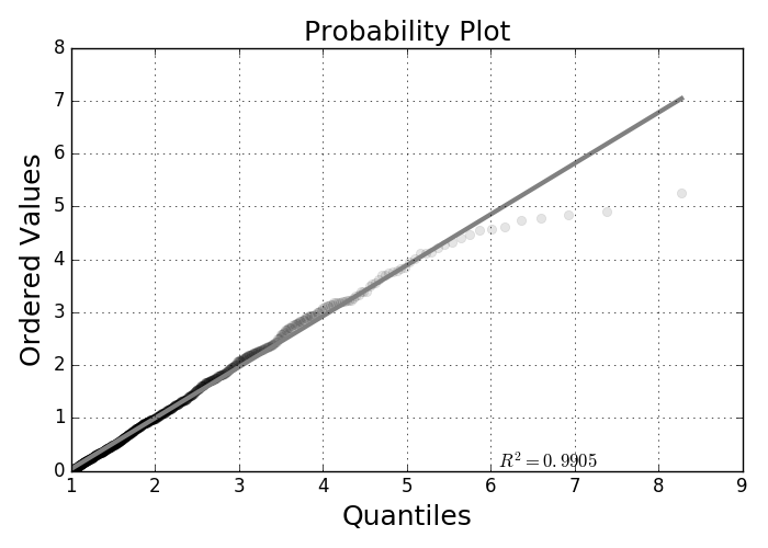
Note that we have to supply an axes object (ax) for it to draw on. The result is Figure. The more the samples line match the diagonal line, the more they match the reference distribution (i.e., exponential distribution in this case). You may also want to try dist=norm in the code above To see what happens when the normal distribution is the reference distribution.

The samples created using the inverse cdf method match the exponential reference distribution.
Rejection Method

In some cases, inverting the CDF may be impossible. The rejection method can handle this situation. The idea is to pick two uniform random variables $u_1,u_2 \sim \mathcal{U}[a,b]$ so that

$$ \mathbb{P}\left(u_1 \in N_{\Delta}(x) \bigwedge u_2 < \frac{f(u_1)}{M} \right) \hspace{0.5em} \approx \frac{\Delta x}{b-a} \frac{f(u_1)}{M} $$

where we take $x=u_1$ and $f(x) < M $. This is a two-step process. First, draw $u_1$ uniformly from the interval $[a,b]$. Second, feed it into $f(x)$ and if $u_2 < f(u_1)/M$, then you have a valid sample for $f(x)$. Thus, $u_1$ is the proposed sample from $f$ that may or may not be rejected depending on $u_2$. The only job of the $M$ constant is to scale down the $f(x)$ so that the $u_2$ variable can span the range. The efficiency of this method is the probability of accepting $u_1$ which comes from integrating out the above approximation,

$$ \int \frac{f(x)}{M(b-a)} dx = \frac{1}{M(b-a)} \int f(x)dx =\frac{1}{M(b-a)} $$

This means that we don't want an unecessarily large $M$ because that makes it more likely that samples will be discarded.

Let's try this method for a density that does not have a continuous inverse 1.

out to one like a probability density function should, but the normalization constant for this is distracting for our purposes here.


  1. Note that this example density does not exactly integrate

$$ f(x) = \exp\left(-\frac{(x-1)^2}{2x} \right) (x+1)/12 $$

where $x>0$. The following code implements the rejection plan.

In [13]:
import numpy as np
x = np.linspace(0.001,15,100)
f= lambda x: np.exp(-(x-1)**2/2./x)*(x+1)/12.
fx = f(x)
M=0.3                          # scale factor
u1 = np.random.rand(10000)*15  # uniform random samples scaled out
u2 = np.random.rand(10000)     # uniform random samples
idx,= np.where(u2<=f(u1)/M)    # rejection criterion
v = u1[idx]
In [14]:
fig,ax=subplots()
fig.set_size_inches((9,5))
_=ax.hist(v,normed=1,bins=40,alpha=.3,color='gray')
_=ax.plot(x,fx,'k',lw=3.,label='$f(x)$')
_=ax.set_title('Estimated Efficency=%3.1f%%'%(100*len(v)/len(u1)),
             fontsize=18)
_=ax.legend(fontsize=18)
_=ax.set_xlabel('$x$',fontsize=24)
fig.tight_layout()
#fig.savefig('fig-probability/Sampling_Monte_Carlo_007.png')

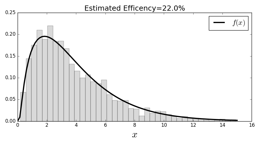
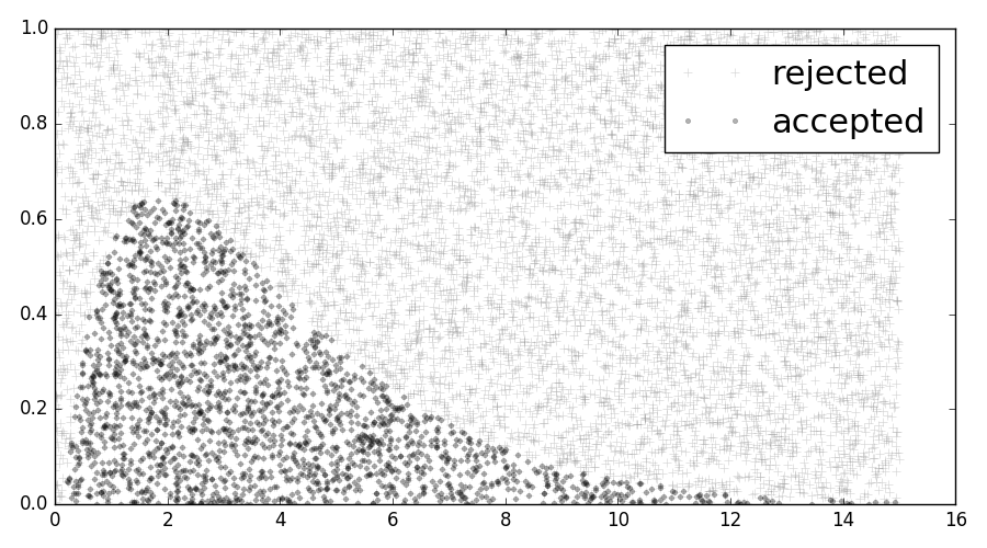
Figure shows a histogram of the so-generated samples that nicely fits the probability density function. The title in the figure shows the efficiency, which is poor. It means that we threw away most of the proposed samples. Thus, even though there is nothing conceptually wrong with this result, the low efficiency must be fixed, as a practical matter. Figure shows where the proposed samples were rejected. Samples under the curve were retained (i.e., $u_2 < \frac{f(u_1)}{M}$) but the vast majority of the samples are outside this umbrella.

The rejection method generate samples in the histogram that nicely match the target distribution. Unfortunately, the efficiency is not so good.
In [15]:
fig,ax=subplots()
fig.set_size_inches((9,5))
_=ax.plot(u1,u2,'+',label='rejected',alpha=.3,color='gray')
_=ax.plot(u1[idx],u2[idx],'.',label='accepted',alpha=.3,color='k')
_=ax.legend(fontsize=22)
fig.tight_layout()
#fig.savefig('fig-probability/Sampling_Monte_Carlo_008.png')

The proposed samples under the curve were accepted and the others were not. This shows the majority of samples were rejected.
The rejection method uses $u_1$ to select along the domain of $f(x)$ and the other $u_2$ uniform random variable decides whether to accept or not. One idea would be to choose $u_1$ so that $x$ values are coincidentally those that are near the peak of $f(x)$, instead of uniformly anywhere in the domain, especially near the tails, which are low probability anyway. Now, the trick is to find a new density function $g(x)$ to sample from that has a similiar concentration of probability density. One way it to familiarize oneself with the probability density functions that have adjustable parameters and fast random sample generators already. There are lots of places to look and, chances are, there is likely already such a generator for your problem. Otherwise, the family of $\beta$ densities is a good place to start.

To be explicit, what we want is $u_1 \sim g(x)$ so that, returning to our earlier argument,

$$ \mathbb{P}\left( u_1 \in N_{\Delta}(x) \bigwedge u_2 < \frac{f(u_1)}{M} \right) \approx g(x) \Delta x \frac{f(u_1)}{M} $$

but this is not what we need here. The problem is with the second part of the logical $\bigwedge$ conjunction. We need to put something there that will give us something proportional to $f(x)$. Let us define the following,

$$ \begin{equation} h(x) = \frac{f(x)}{g(x)} \end{equation} \label{eq:rej01} \tag{2} $$

with corresponding maximum on the domain as $h_{\max}$ and then go back and construct the second part of the clause as

$$ \mathbb{P}\left(u_1 \in N_{\Delta}(x) \bigwedge u_2 < \frac{h(u_1)}{h_{\max}} \right) \approx g(x) \Delta x \frac{h(u_1)}{h_{\max}} = f(x)/h_{\max} $$

Recall that satisfying this criterion means that $u_1=x$. As before, we can estimate the probability of acceptance of the $u_1$ as $1/h_{\max}$.

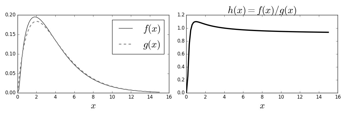
Now, how to construct the $g(x)$ function in the denominator of Equation ref{eq:rej01}? Here's where familarity with some standard probability densities pays off. For this case, we choose the chi-squared distribution. The following plots the $g(x)$ and $f(x)$ (left plot) and the corresponding $h(x)=f(x)/g(x)$ (right plot). Note that $g(x)$ and $f(x)$ have peaks that almost coincide, which is what we are looking for.

In [16]:
ch=scipy.stats.chi2(4) # chi-squared
h = lambda x: f(x)/ch.pdf(x) # h-function
In [17]:
fig,axs=subplots(1,2,sharex=True)
fig.set_size_inches(12,4)
_=axs[0].plot(x,fx,label='$f(x)$',color='k')
_=axs[0].plot(x,ch.pdf(x),'--',lw=2,label='$g(x)$',color='gray')
_=axs[0].legend(loc=0,fontsize=24)
_=axs[0].set_xlabel(r'$x$',fontsize=22)
_=axs[1].plot(x,h(x),'-k',lw=3)
_=axs[1].set_title('$h(x)=f(x)/g(x)$',fontsize=24)
_=axs[1].set_xlabel(r'$x$',fontsize=22)
fig.tight_layout()
#fig.savefig('fig-probability/Sampling_Monte_Carlo_009.png')

The plot on the right shows $h(x)=f(x)/g(x)$ and the one on the left shows $f(x)$ and $g(x)$ separately.
Now, let's generate some samples from this $\chi^2$ distribution with the rejection method.

In [18]:
hmax=h(x).max()
u1 = ch.rvs(5000)        # samples from chi-square distribution
u2 = np.random.rand(5000)# uniform random samples
idx = (u2 <= h(u1)/hmax) # rejection criterion
v = u1[idx]              # keep these only
In [19]:
fig,ax=subplots()
fig.set_size_inches((7,3))
_=ax.hist(v,normed=1,bins=40,alpha=.3,color='gray')
_=ax.plot(x,fx,color='k',lw=3.,label='$f(x)$')
_=ax.set_title('Estimated Efficency=%3.1f%%'%(100*len(v)/len(u1)))
_=ax.axis(xmax=15)
_=ax.legend(fontsize=18)
#fig.savefig('fig-probability/Sampling_Monte_Carlo_010.png')

Using the updated method, the histogram matches the target probability density function with high efficiency.
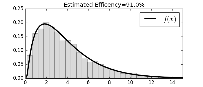
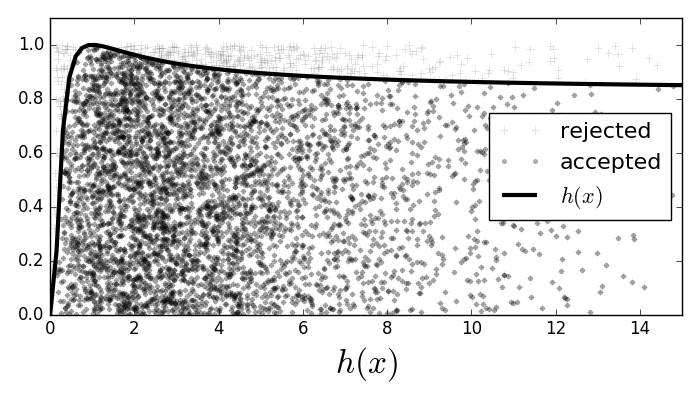
Using the $\chi^2$ distribution with the rejection method results in throwing away less than 10% of the generated samples compared with our prior example where we threw out at least 80%. This is dramatically more efficient. Figure shows that the histogram and the probability density function match. For completeness, Figure shows the samples with the corresponding threshold $h(x)/h_{\max}$ that was used to select them.

In [20]:
fig,ax=subplots()
fig.set_size_inches((7,4))
_=ax.plot(u1,u2,'+',label='rejected',alpha=.3,color='gray')
_=ax.plot(u1[idx],u2[idx],'g.',label='accepted',alpha=.3,color='k')
_=ax.plot(x,h(x)/hmax,color='k',lw=3.,label='$h(x)$')
_=ax.legend(fontsize=16,loc=0) 
_=ax.set_xlabel('$x$',fontsize=24)
_=ax.set_xlabel('$h(x)$',fontsize=24)
_=ax.axis(xmax=15,ymax=1.1)
fig.tight_layout()
#fig.savefig('fig-probability/Sampling_Monte_Carlo_011.png')

Fewer proposed points were rejected in this case, which means better efficiency.
In this section, we investigated how to generate random samples from a given distribution, beit discrete or continuous. For the continuous case, the key issue was whether or not the cumulative density function had a continuous inverse. If not, we had to turn to the rejection method, and find an appropriate related density that we could easily sample from to use as part of a rejection threshold. Finding such a function is an art, but many families of probability densities have been studied over the years that already have fast random number generators.

The rejection method has many complicated extensions that involve careful partitioning of the domains and lots of special methods for corner cases. Nonetheless, all of these advanced techniques are still variations on the same fundamental theme we illustrated here [dunn2011exploring],[johnson1995continuous].