from IPython.display import Image
Image('../../../python_for_probability_statistics_and_machine_learning.jpg')
Projection Methods
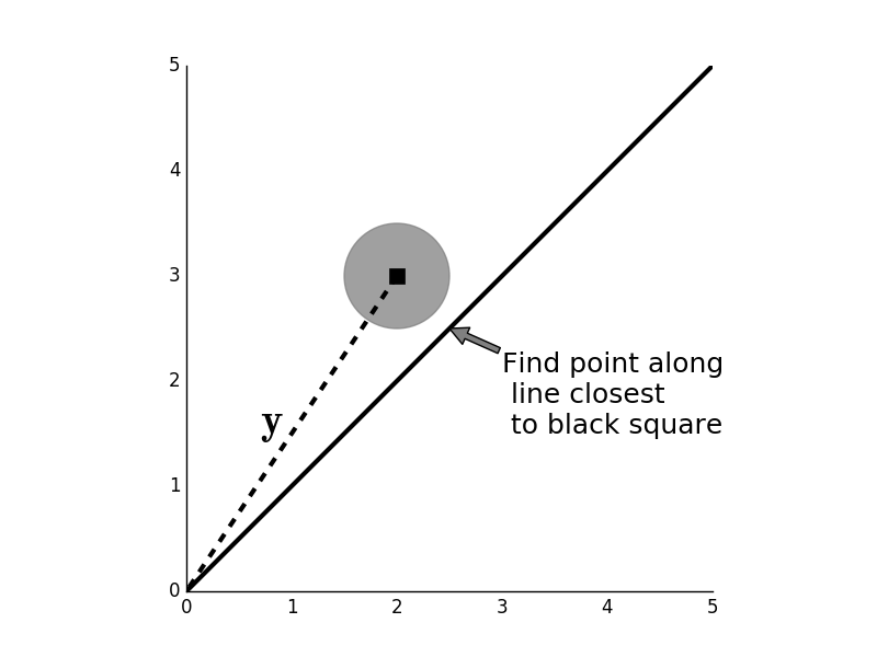
The concept of projection is key to developing an intuition about conditional probability. We already have a natural intuition of projection from looking at the shadows of objects on a sunny day. As we will see, this simple idea consolidates many abstract ideas in optimization and mathematics. Consider Figure where we want to find a point along the blue line (namely, $\mathbf{x}$) that is closest to the black square (namely, $\mathbf{y}$). In other words, we want to inflate the gray circle until it just touches the black line. Recall that the circle boundary is the set of points for which
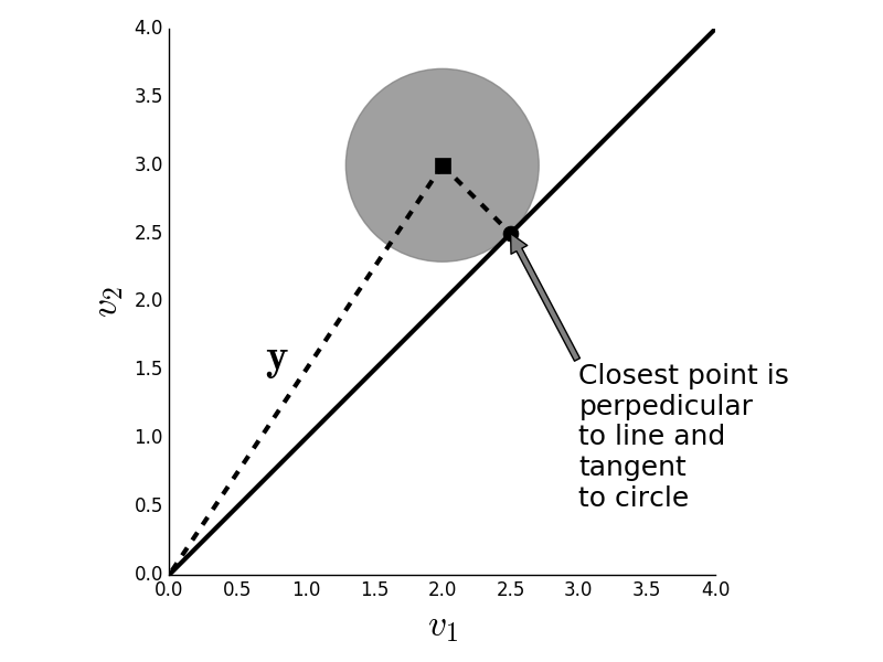
for some value of $\epsilon$. So we want a point $\mathbf{x}$ along the line that satisfies this for the smallest $\epsilon$. Then, that point will be the closest point on the black line to the black square. It may be obvious from the diagram, but the closest point on the line occurs where the line segment from the black square to the black line is perpedicular to the line. At this point, the gray circle just touches the black line. This is illustrated below in Figure.
Given the point $\mathbf{y}$ (black square) we want to find the $\mathbf{x}$ along the line that is closest to it. The gray circle is the locus of points within a fixed distance from $\mathbf{y}$.

Programming Tip.
Figure uses the matplotlib.patches module. This
module contains primitive shapes like circles, ellipses, and rectangles that
can be assembled into complex graphics. As shown in the code in the IPython
Notebook corresponding to this chapter, after importing a particular shape, you
can apply that shape to an existing axis using the add_patch method. The
patches themselves can by styled using the usual formatting keywords like
color and alpha.
The closest point on the line occurs when the line is tangent to the circle. When this happens, the black line and the line (minimum distance) are perpedicular.

Now that we can see what's going on, we can construct the the solution analytically. We can represent an arbitrary point along the black line as:
where $\alpha\in\mathbb{R}$ slides the point up and down the line with
Formally, $\mathbf{v}$ is the subspace onto which we want to project $\mathbf{y}$. At the closest point, the vector between $\mathbf{y}$ and $\mathbf{x}$ (the error vector above) is perpedicular to the line. This means that
and by substituting and working out the terms, we obtain
The error is the distance between $\alpha\mathbf{v}$ and $ \mathbf{y}$. This is a right triangle, and we can use the Pythagorean theorem to compute the squared length of this error as
where $ \|\mathbf{v}\|^2 = \mathbf{v}^T \mathbf{v} $. Note that since $\epsilon^2 \ge 0 $, this also shows that
which is the famous and useful Cauchy-Schwarz inequality which we will exploit later. Finally, we can assemble all of this into the projection operator
With this operator, we can take any $\mathbf{y}$ and find the closest point on $\mathbf{v}$ by doing
where we recognize the term in parenthesis as the $\alpha$ we computed earlier. It's called an operator because it takes a vector ($\mathbf{y}$) and produces another vector ($\alpha\mathbf{v}$). Thus, projection unifies geometry and optimization.
Weighted distance
We can easily extend this projection operator to cases where the measure of distance between $\mathbf{y}$ and the subspace $\mathbf{v}$ is weighted. We can accommodate these weighted distances by re-writing the projection operator as
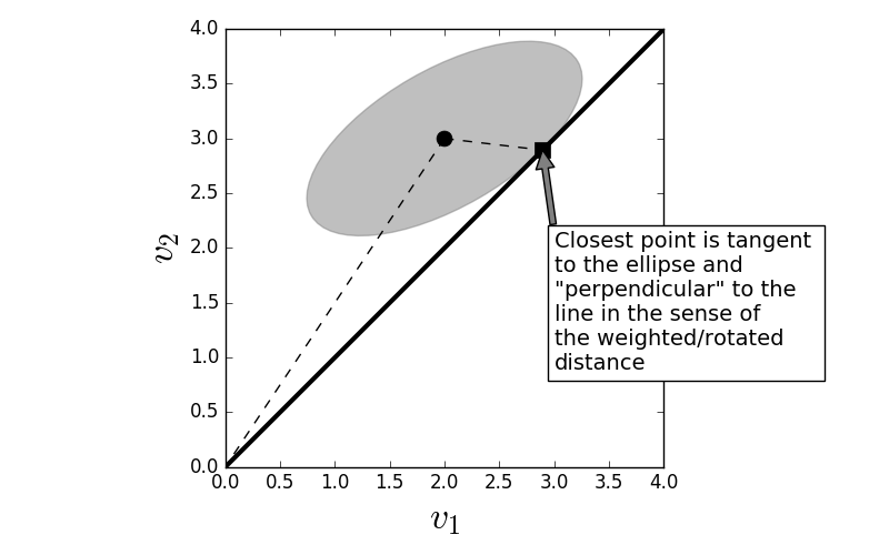
where $\mathbf{Q}$ is positive definite matrix. In the previous case, we started with a point $\mathbf{y}$ and inflated a circle centered at $\mathbf{y}$ until it just touched the line defined by $\mathbf{v}$ and this point was closest point on the line to $\mathbf{y}$. The same thing happens in the general case with a weighted distance except now we inflate an ellipse, not a circle, until the ellipse touches the line.
In the weighted case, the closest point on the line is tangent to the ellipse and is still perpedicular in the sense of the weighted distance.

Note that the error vector ($\mathbf{y}-\alpha\mathbf{v}$) in Figure is still perpendicular to the line (subspace $\mathbf{v}$), but in the space of the weighted distance. The difference between the first projection (with the uniform circular distance) and the general case (with the elliptical weighted distance) is the inner product between the two cases. For example, in the first case we have $\mathbf{y}^T \mathbf{v}$ and in the weighted case we have $\mathbf{y}^T \mathbf{Q}^T \mathbf{v}$. To move from the uniform circular case to the weighted ellipsoidal case, all we had to do was change all of the vector inner products. Before we finish, we need a formal property of projections:
known as the idempotent property which basically says that once we have projected onto a subspace, subsequent projections leave us in the same subspace. You can verify this by computing Equation ref{eq:weightedProj}.
Thus, projection ties a minimization problem (closest point to a line) to an algebraic concept (inner product). It turns out that these same geometric ideas from linear algebra [strang2006linear] can be translated to the conditional expectation. How this works is the subject of our next section.