from IPython.display import Image
Image('../../../python_for_probability_statistics_and_machine_learning.jpg')
from __future__ import division
%pylab inline
In a previous coin-flipping discussion, we discussed estimation of the underlying probability of getting a heads. There, we derived the estimator as
where $X_i\in \lbrace 0,1 \rbrace$. Confidence intervals allow us to estimate how close we can get to the true value that we are estimating. Logically, that seems strange, doesn't it? We really don't know the exact value of what we are estimating (otherwise, why estimate it?), and yet, somehow we know how close we can get to something we admit we don't know? Ultimately, we want to make statements like the probability of the value in a certain interval is 90\%. Unfortunately, that is something we will not be able to say using our methods. Note that Bayesian estimation gets closer to this statement by using credible intervals, but that is a story for another day. In our situation, the best we can do is say roughly the following: if we ran the experiment multiple times, then the confidence interval would trap the true parameter 90\% of the time.
Let's return to our coin-flipping example and see this in action. One way to get at a confidence interval is to use Hoeffding's inequality from the section ref{ch:prob:sec:ineq} specialized to our Bernoulli variables as
Now, we can form the interval $\mathbb{I}=[\hat{p}_n-\epsilon_n,\hat{p}_n+\epsilon_n]$, where $\epsilon_n$ is carefully constructed as
which makes the right-side of the Hoeffding inequality equal to $\alpha$. Thus, we finally have
Thus, $ \mathbb{P}(p \in \mathbb{I}) \geq 1-\alpha$. As a numerical example, let's take $n=100$, $\alpha=0.05$, then plugging into everything we have gives $\epsilon_n=0.136$. So, the 95\% confidence interval here is therefore
The following code sample is a simulation to see if we can really trap the underlying parameter in our confidence interval.
from scipy import stats
import numpy as np

b= stats.bernoulli(.5) # fair coin distribution
nsamples = 100
# flip it nsamples times for 200 estimates
xs = b.rvs(nsamples*200).reshape(nsamples,-1)
phat = np.mean(xs,axis=0) # estimated p
# edge of 95% confidence interval
epsilon_n=np.sqrt(np.log(2/0.05)/2/nsamples)
pct=np.logical_and(phat-epsilon_n<=0.5,
                   0.5 <= (epsilon_n +phat)
                   ).mean()*100
print 'Interval trapped correct value ', pct,'% of the time'
The result shows that the estimator and the corresponding interval was able to trap the true value at least 95\% of the time. This is how to interpret the action of confidence intervals.
However, the usual practice is to not use Hoeffding's inequality and instead use arguments around asymptotic normality. The definition of the standard error is the following:
where $\hat{\theta}_n$ is the point-estimator for the parameter $\theta$, given $n$ samples of data $X_n$, and $\mathbb{V}(\hat{\theta}_n)$ is the variance of $\hat{\theta}_n$. Likewise, the estimated standard error is $\widehat{\texttt{se}}$. For example, in our coin-flipping example, the estimator was $\hat{p}=\sum X_i/n$ with corresponding variance $\mathbb{V}(\hat{p}_n)=p(1-p)/n$. Plugging in the point estimate gives us the estimated standard error: $\widehat{\texttt{se}}=\sqrt{\hat{p}(1-\hat{p})/n}$. Because maximum likelihood estimators are asymptotically normal 1, we know that $\hat{p}_n \sim \mathcal{N}(p,\widehat{\texttt{se}}^2)$. Thus, if we want a $1-\alpha$ confidence interval, we can compute
of maximum likelihood estimator to work. See [wasserman2004all] for more details.
Certain technical regularity conditions must hold for this property↩
but since we know that $ (\hat{p}_n-p)$ is asymptotically normal, $\mathcal{N}(0,\widehat{\texttt{se}}^2)$, we can instead compute
This looks ugly to compute because we need to find $\xi$, but Scipy has everything we need for this.
# compute estimated se for all trials
se=np.sqrt(phat*(1-phat)/xs.shape[0])
# generate random variable for trial 0
rv=stats.norm(0, se[0])
# compute 95% confidence interval for that trial 0
np.array(rv.interval(0.95))+phat[0]
def compute_CI(i):
    return stats.norm.interval(0.95,loc=i,
                              scale=np.sqrt(i*(1-i)/xs.shape[0]))

lower,upper = compute_CI(phat)
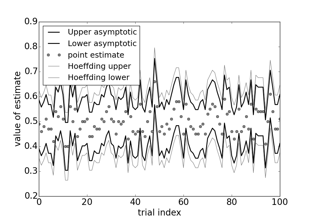
The gray circles are the point estimates that are bounded above and below by both asymptotic confidence intervals and Hoeffding intervals. The asymptotic intervals are tighter because the underpinning asymptotic assumptions are valid for these estimates.

Figure shows the asymptotic confidence intervals and the Hoeffding-derived confidence intervals. As shown, the Hoeffding intervals are a bit more generous than the asymptotic estimates. However, this is only true so long as the asympotic approximation is valid. In other words, there exists some number of $n$ samples for which the asymptotic intervals may not work. So, even though they may be a bit more generous, the Hoeffding intervals do not require arguments about asymptotic convergence. In practice, nonetheless, asymptotic convergence is always in play (even if not explicitly stated).
Confidence Intervals and Hypothesis testing
It turns out that there is a close dual relationship between hypothesis testing and confidence intervals. To see this in action, consider the following hypothesis test for a normal distribution, $H_0 :\mu=\mu_0$ versus $H_1: \mu \neq \mu_0$. A reasonable test has the following rejection region:
where $\mathbb{P}(Z > z_{\alpha/2}) = \alpha/2$ and $\mathbb{P}(-z_{\alpha/2}< Z < z_{\alpha/2}) = 1-\alpha$ and where $Z \sim \mathcal{N}(0,1)$. This is the same thing as saying that the region corresponding to acceptance of $H_0$ is then,
Because the test has size $\alpha$, the false alarm probability, $\mathbb{P}(H_0 \texttt{ rejected}\mid \mu=\mu_0)=\alpha$. Likewise, the $\mathbb{P}(H_0 \texttt{ accepted}\mid \mu=\mu_0)=1-\alpha$. Putting this all together with interval defined above means that
Because this is valid for any $\mu_0$, we can drop the $H_0$ condition and say the following:
As may be obvious by now, the interval in Equation ref{eq:ci} above is the $1-\alpha$ confidence interval! Thus, we have just obtained the confidence interval by inverting the acceptance region of the level $\alpha$ test. The hypothesis test fixes the parameter and then asks what sample values (i.e., the acceptance region) are consistent with that fixed value. Alternatively, the confidence interval fixes the sample value and then asks what parameter values (i.e., the confidence interval) make this sample value most plausible. Note that sometimes this inversion method results in disjoint intervals (known as confidence sets).