from IPython.display import Image
Image('../../../python_for_probability_statistics_and_machine_learning.jpg')
from __future__ import division
%pylab inline
In this section, we consider the famous Gauss-Markov problem which will give us an opportunity to use all the material we have so far developed. The Gauss-Markov model is the fundamental model for noisy parameter estimation because it estimates unobservable parameters given a noisy indirect measurement. Incarnations of the same model appear in all studies of Gaussian models. This case is an excellent opportunity to use everything we have so far learned about projection and conditional expectation.
Following Luenberger [luenberger1968optimization] let's consider the following problem:
where $\mathbf{W}$ is a $ n \times m $ matrix, and $\mathbf{y}$ is a $n \times 1$ vector. Also, $\boldsymbol{\epsilon}$ is a $n$-dimensional normally distributed random vector with zero-mean and covariance,
Note that engineering systems usually provide a calibration mode where you can estimate $\mathbf{Q}$ so it's not fantastical to assume you have some knowledge of the noise statistics. The problem is to find a matrix $\mathbf{K}$ so that $ \boldsymbol{\hat{\beta}}=\mathbf{K} \mathbf{y}$ approximates $ \boldsymbol{\beta}$. Note that we only have knowledge of $\boldsymbol{\beta}$ via $ \mathbf{y}$ so we can't measure it directly. Further, note that $\mathbf{K} $ is a matrix, not a vector, so there are $m \times n$ entries to compute.
We can approach this problem the usual way by trying to solve the MMSE problem:
which we can write out as
and since $\boldsymbol{\epsilon}$ is the only random variable here, this simplifies to
The next step is to compute
using the properties of the trace of a matrix. We can assemble everything as
Now, if we were to solve this for $\mathbf{K}$, it would be a function of $ \boldsymbol{\beta}$, which is the same thing as saying that the estimator, $ \boldsymbol{\hat{\beta}}$, is a function of what we are trying to estimate, $\boldsymbol{\beta}$, which makes no sense. However, writing this out tells us that if we had $\mathbf{K W}= \mathbf{I}$, then the first term vanishes and the problem simplifies to
with the contraint,
This requirement is the same as asserting that the estimator is unbiased,
To line this problem up with our earlier work, let's consider the $i^{th}$ column of $\mathbf{K}$, $\mathbf{k}_i$. Now, we can re-write the problem as
with
and from our previous work on contrained optimization, we know the solution to this:
Now all we have to do is stack these together for the general solution:
It's easy when you have all of the concepts lined up! For completeness, the covariance of the error is
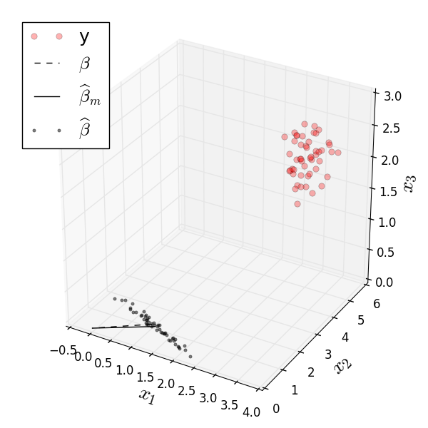
The red circles show the points to be estimated in the xy-plane by the black points.

Figure shows the simulated $\mathbf{y}$ data as red circles. The black dots show the corresponding estimates, $\boldsymbol{\hat{\beta}}$ for each sample. The black lines show the true value of $\boldsymbol{\beta}$ versus the average of the estimated $\boldsymbol{\beta}$-values, $\widehat{\boldsymbol{\beta}_m}$. The matrix $\mathbf{K}$ maps the red circles in the corresponding dots. Note there are many possible ways to map the red circles to the plane, but the $\mathbf{K}$ is the one that minimizes the MSE for $\boldsymbol{\beta}$.
Programming Tip.
Although the full source code is available in the corresponding IPython Notebook, the following snippets provide a quick walkthrough. To simulate the target data, we define the relevant matrices below,
Q = np.eye(3)*0.1 # error covariance matrix
# this is what we are trying estimate
beta = matrix(ones((2,1)))
W = matrix([[1,2],
            [2,3],
            [1,1]])
Then, we generate the noise terms and create the simulated data, $y$,
ntrials = 50
epsilon = np.random.multivariate_normal((0,0,0),Q,ntrials).T
y=W*beta+epsilon
Focusing on the xy-plane in [Figure](#fig:Gauss_Markov_001), the dashed line shows the true value for $\boldsymbol{\beta}$ versus the mean of the estimated values $\widehat{\boldsymbol{\beta}}_m$.

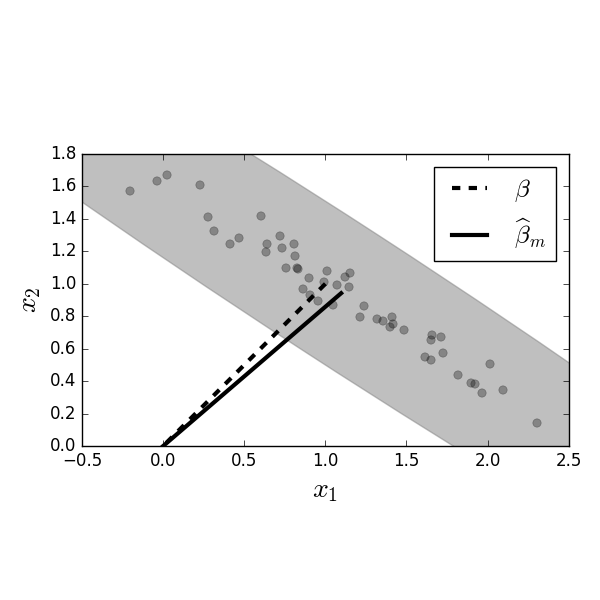
Figure shows more detail in the horizontal xy-plane of Figure. Figure shows the dots, which are individual estimates of $\boldsymbol{\hat{\beta}}$ from the corresponding simulated $\mathbf{y}$ data. The dashed line is the true value for $\boldsymbol{\beta}$ and the filled line ($\widehat{\boldsymbol{\beta}}_m$) is the average of all the dots. The gray ellipse provides an error ellipse for the covariance of the estimated $\boldsymbol{\beta}$ values.
Programming Tip.
Although the full source code is available in the corresponding IPython Notebook, the following snippets provide a quick walkthrough of the construction of Figure. To draw the ellipse, we need to import the patch primitive,
# %matplotlib inline

# from  matplotlib.patches import Ellipse
To compute the parameters of the error ellipse based on the
covariance matrix of the individual estimates of $\boldsymbol{\beta}$
in the bm_cov variable below,
# U,S,V = linalg.svd(bm_cov)
# err = np.sqrt((matrix(bm))*(bm_cov)*(matrix(bm).T))
# theta = np.arccos(U[0,1])/np.pi*180
Then, we draw the add the scaled ellipse in the following,
# ax.add_patch(Ellipse(bm,err*2/np.sqrt(S[0]),
#                      err*2/np.sqrt(S[1]),
#                      angle=theta,color='gray'))
from __future__ import division
from mpl_toolkits.mplot3d import proj3d
from numpy.linalg import inv
import matplotlib.pyplot as plt
import numpy as np
from numpy import matrix, linalg, ones, array

Q = np.eye(3)*.1 # error covariance matrix

beta = matrix(ones((2,1))) # this is what we are trying estimate
W = matrix([[1,2],
            [2,3],
            [1,1]])

ntrials = 50
epsilon = np.random.multivariate_normal((0,0,0),Q,ntrials).T
y=W*beta+epsilon

K=inv(W.T*inv(Q)*W)*matrix(W.T)*inv(Q)
b=K*y #estimated beta from data

fig = plt.figure()
fig.set_size_inches([6,6])

# some convenience definitions for plotting
bb = array(b)
bm = bb.mean(1)
yy = array(y)
ax = fig.add_subplot(111, projection='3d')

ax.plot3D(yy[0,:],yy[1,:],yy[2,:],'ro',label='y',alpha=0.3)
ax.plot3D([beta[0,0],0],[beta[1,0],0],[0,0],'k--',label=r'$\beta$')
ax.plot3D([bm[0],0],[bm[1],0],[0,0],'k-',lw=1,label=r'$\widehat{\beta}_m$')
ax.plot3D(bb[0,:],bb[1,:],0*bb[1,:],'.k',alpha=0.5,lw=3,label=r'$\widehat{\beta}$')
ax.legend(loc=0,fontsize=18)
ax.set_xlabel('$x_1$',fontsize=20)
ax.set_ylabel('$x_2$',fontsize=20)
ax.set_zlabel('$x_3$',fontsize=20)
fig.tight_layout()

from  matplotlib.patches import Ellipse

fig, ax = plt.subplots()
fig.set_size_inches((6,6))
ax.set_aspect(1)
ax.plot(bb[0,:],bb[1,:],'ko',alpha=.3)
ax.plot([beta[0,0],0],[beta[1,0],0],'k--',label=r'$\beta$',lw=3)
ax.plot([bm[0],0],[bm[1],0],'k-',lw=3,label=r'$\widehat{\beta}_m$')
ax.legend(loc=0,fontsize=18)

bm_cov = inv(W.T*Q*W)
U,S,V = linalg.svd(bm_cov)

err = np.sqrt((matrix(bm))*(bm_cov)*(matrix(bm).T))
theta = np.arccos(U[0,1])/np.pi*180

ax.add_patch(Ellipse(bm,err*2/np.sqrt(S[0]),err*2/np.sqrt(S[1])
                       ,angle=theta,color='gray',alpha=0.5))

ax.set_xlabel('$x_1$',fontsize=20)
ax.set_ylabel('$x_2$',fontsize=20)
fig.tight_layout()